1. Honey Dataset
For the selected honey samples after microscopy analysis and sensory assessment, a dataset was built using the mean values of each determination. The dataset is summarized in
Figures S1 and S2 (https://www.mdpi.com/article/10.3390/foods10071543/s1). After microscopic analysis, pollen count was related to nectariferous plants. The box plots of percentages of pollen from the taxa that give the names to the studied unifloral honeys are shown in
Figure S2g. Selected samples were as follows: Rosemary honeys that had 20–77% pollen from
R. officinalis were considered acceptable as it is known as an under-represented pollen. Orange blossom or citrus honeys had a percentage of
Citrus spp. pollen in the range 10–46%, except in one sample (80%). Citrus honeys are considered unifloral if the pollen of
Citrus spp. is >10% because it is considered as under-represented. Lavender honeys sowed a percentage of
Lavandula latifolia or
L. spica in the range 15–68%. Pollen from
L. stoechas was usually absent. Additionally, in this honey class, the pollen is considered under-represented. Sunflower honeys had pollen of
H. annuus in the range 31‒82%. Eucalyptus honeys contained 82‒98% pollen of
Eucalyptus spp. High counts in this case are usual because
Eucalyptus pollen is over-represented. Heather honeys encompassed pollen from
Erica spp. in the range 48–80% (
Figure S2g). For forest honey, which is mainly honeydew honey, pollen counts of
Quercus spp., although always present, are of no interest, as previously commented, because their flowers are non-nectariferous, but they were always examined microscopically for HDE and the presence of pollen from other taxa. HDE presence was scarce. Concerning organoleptic properties, rosemary and orange honeys displayed a light amber color and had a characteristic aroma and taste. Lavender and eucalyptus honeys were light amber but darker than orange or rosemary honeys and had a characteristic aroma and taste. Sunflower honeys had a yellow characteristic and a bright golden-amber color, with a yellow hue and slight tart aroma, and crystalized easily, producing fine crystals. Heather honeys were amber/dark amber with a reddish hue and had a characteristic intense aroma and sour taste and a tendency to crystallize. Forest honeys were also dark amber/dark, had an intense flavor, were slightly bitter and sour and remained liquid even in cool conditions for months.
Figures S1 and S2 show the large variability of the data. Some rosemary and citrus honeys had a high moisture percentage, and the lower water levels were found in eucalyptus and forest honeys, while the remaining honey types exhibited intermediate water contents (
Figure S1a). All lavender honeys were well below the 15% limit for sucrose established in the EU Council directive
[1]. Forest and heather honeys showed the highest values of electrical conductivity, followed by eucalyptus and lavender/sunflower honeys, while rosemary and citrus displayed the lowest values for this parameter (
Figure S1). The pH was also higher in forest and heather honeys than in the remaining honeys. The highest contents of fructose and glucose and the highest glucose/water ratio were found in sunflower honeys, which also had the lowest fructose/glucose ratio; forest honeys showed the lowest levels of both fructose and glucose. On the contrary, maltose, isomaltose and kojibiose contents and the fructose/glucose ratio reached the highest values in forest honeys (
Figures S1 and S2). Concerning the color parameters, the largest x values were observed in heather honeys followed by forest honeys, and the minimum x values were observed in rosemary and citrus honeys. However, heather honeys had the lowest mean value for the y and L chromatic coordinates. The largest mean y value was exhibited by sunflowers honeys, and the largest mean L value was observed in citrus honeys (
Figure S2).
2. Statistical and ML Algorithms
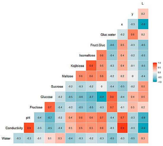
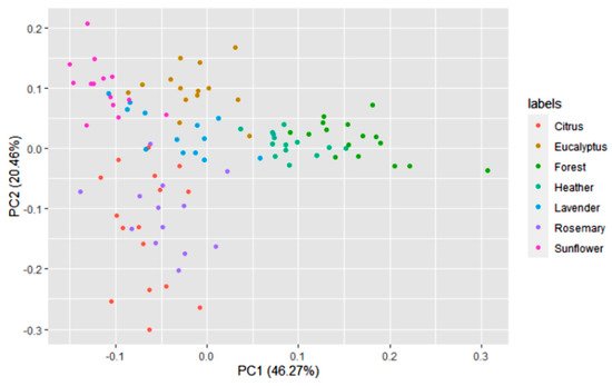
A multivariate statistical study of the dataset was carried out initially. Variables were centered and scaled before statistical treatments. Correlations, PCA and data clustering were performed. A diagram including correlations between all the variables is shown in Figure 1. A score plot of the two principal components can be observed in Figure 2. PC1 and PC2 account for 45.27% and 20.46% of the variance, respectively (overall 66.73%). Heather and forest honeys spread along the positive side of PC1. Sunflower honeys extend on the negative side of PC1, but on the positive side of PC2. All citrus and most rosemary honeys are on the negative side of both PC1 and PC2. Eucalyptus honey samples spread on the positive side of PC2, and most of them are on the negative side of PC1, while most lavender honeys fall on the negative side of PC1, but they spread on both the positive and negative sides of PC2.
Figure 1. Correlation chart among the 14 predictor variables for the whole dataset. The number in each square is rounded to one figure. The color scale at the right indicates color meaning. Red color means positive correlation; blue color means negative correlation.
Figure 2. Principal component score plot based on the 14 variables of 100 honey samples according to the botanical origins.
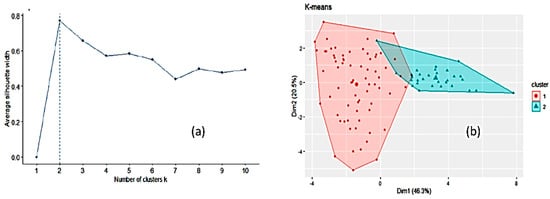
Another unsupervised way to explore the dataset, k-means clustering
[2][3], was run to partition the data into a number of clusters using the library “factoextra” in R. All the input variables were taken into account. Two clusters of sizes 70 and 30 were obtained on the basis of the maximum average silhouette width (
Figure 3). However, this number of clusters is an estimate and does not mean that only two clusters may exist. The mean values for the variables in each of these two clusters (corresponding to the centroids) are listed in
Table S1. Cluster 2 is smaller in size than cluster 1 and is higher than cluster 1 in mean values of electrical conductivity, pH, disaccharides (except sucrose), fructose/glucose ratio and the x chromatic coordinate. When comparing
Figure 2 and
Figure 3b, cluster 2 seems to encompass forest and heather honeys and cluster 1 the remaining honeys. Forcing the k-means clustering to display seven groups on a two-dimensional plot leads to highly overlapped clusters (
Figure S3). The relative importance of the variables was tested using an RF model as a reference (
Figure S4). The most important variables are electrical conductivity, the chromatic coordinates, water content, fructose and glucose. The less important variables are glucose/water and fructose/glucose ratios. The Boruta package
[4] was applied, and it considered that no variables had to be removed regardless of their relative importance.
Figure 3. Optimal number of clusters by k-means using the average silhouette width (a) and clustering of honey samples by k-means algorithm in two clusters where the two largest symbols are the centroids of each cluster (b).
Using the approach of supervised modeling, different classifier algorithms were applied to the dataset, which was divided into a training set (70%) and a test set (30%). Ten-fold cross-validation was applied during training with four repetitions. Various metrics (log loss, accuracy, AUC, kappa, sensitivity, specificity, precision, etc.) can be used during training to tune the key parameters of the algorithms in order to find the best ones. The absolute values of metrics vary when training is repeated. Among them, the log loss metric was usually chosen to select the optimal model using the smallest value. For KKNN or KNN (as weights were not relevant), the final value of the tuning parameters used for the optimized model was kmax (maximum number of neighbors) = 5 (Table 1).
Table 1. Model optimization using the classifier algorithms. Log loss values are means of 10-fold cross-validation.
| Algorithm |
Tuning Parameter |
Mean Log Loss Values |
| KKNN |
Kmax = 5 |
0.8339319 |
| Kmax = 7 |
0.9017721 |
| Kmax = 9 |
0.9808674 |
| PDA |
Lambda = 1 |
0.5689435 |
| Lambda = 0.0001 |
0.5687306 |
| Lambda = 0.1 |
0.4611719 |
| HDDA |
Thershold = 0.05 |
0.4360396 |
| Thershold = 0.175 |
1.3732500 |
| Thershold = 0.300 |
1.0080708 |
| SDA |
Lambda = 0.0 |
0.6320813 |
| Lambda = 0.5 |
0.3968958 |
| Lambda = 1.0 |
0.4908678 |
| PAM |
Threshold = 0.7608929 |
0.4986565 |
| Threshold = 11.0329476 |
1.9483062 |
| Threshold = 21.3050022 |
1.9483062 |
| PLS |
Ncomp = 1 |
1.826913 |
| Ncomp = 2 |
1.733439 |
| Ncomp = 3 |
1.643669 |
| C5.0 tree |
|
0.7482527 |
| ET |
|
0.3590714 |
For the PDA algorithm, the optimal lambda value was 0.1. For HDDA, the best model had a threshold of 0.300, but this algorithm is not robust and other repetitions led to a different configuration; for SDA, the lowest log loss was obtained with lambda = 0.05, and for PAM, the best model had a threshold = 0.70615. This value can change slightly if the whole treatment is repeated. With PLS, log loss was also used to select the optimal model using the smallest value, and the final value selected for the model was as follows: number of components (ncomp) = 3 (Table 1).
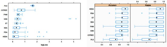
The box plots for the three main metric parameters log loss, accuracy and kappa for eight classifiers can be observed in Figure 4.
Figure 4. Box plots of log loss, accuracy and kappa values for various machine learning (ML) algorithms after training with 10-fold cross-validation to obtain the best model using the training dataset. Black circles symbolize mean values. PLS: partial least squares; C5TREE: C5.0 tree; PAM: nearest shrunken centroids; KNN: weighted k-nearest neighbors; ET: extremely randomized trees; SDA: shrinkage discriminant analysis; PDA: penalized discriminant analysis; HDDA: high-dimensional discriminant analysis.
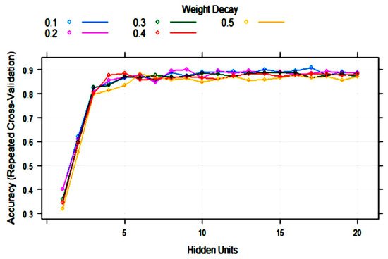
ANN (single-layer perceptron) was applied to the training set with 10-fold cross-validation. The training process evaluated from 1 to 20 hidden units (neurons) and weight decays from 0.1 to 0.5. After optimization of tuning parameters to maximize the validation accuracy, the best model had 17 hidden units and weight decay = 0.1 (Figure 5). As it can be observed, the variability of accuracy with more than five hidden units is low, ranging from 0.85 to 0.91. This means that repetitions of the treatments can produce different topologies with very similar accuracy.
Figure 5. Change in the artificial neural network (ANN) accuracy during training with 10-fold cross-validation with the number of hidden units (nodes) and weight decay.
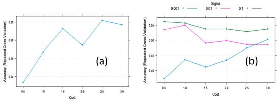
The accuracy of the SVM with linear kernels (SVML) algorithm during training with 10-fold cross-validation was maximized, with a value of the cost function of C = 2.5 (Figure 6). The largest value of the accuracy (0.61) was relatively low. In an attempt to improve SVM, we tested SVM with radial basis function kernels (SVMR). The final values used for the SVMR model were sigma = 0.1 and C = 0.5 (Figure 6). The accuracy was 0.562, meaning it was not improved. However, the cost value of these algorithms was quite variable on repeated treatments, maintaining the same partition ratio.
Figure 6. Change in accuracy of (a) Support vector machine with linear kernel (SVML) and (b) Support vector machine with radial kernel (SVMR) during training with 10-fold cross-validation (CV) with the cost function.
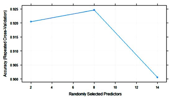
Figure 7 shows the variation in RF accuracy throughout training with 10-fold cross-validation. The final values for the RF model were as follows: number of variables randomly sampled as candidates at each split (mtry) = 8; the number of trees (ntry) parameter was 500; the maximum accuracy was 0.9246.
Figure 7. Change in the accuracy of random forest (RF) models with the number of randomly selected predictors (mtry).
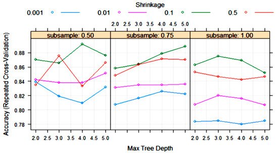
The XGBoost tree algorithm has many parameters to tune, although, usually, some of them are held constant. Figure 8 shows the variation in some tuning parameters during the training process. The largest accuracy was obtained with “subsample” = 0.5, “shrinkage (eta)” = 0.1 and “max tree depth” = 4. Other final values for the model were “nrounds” = 200, “gamma” = 0, “colsample_bytree” = 0.8 and “min_child_weight” = 1.
Figure 8. Change in the accuracy of XGBoost algorithm during training with 10-fold cross-validation with the parameters “max tree depth”, “shrinkage (eta)” and “subsample”. Tuning parameters “nrounds”, “gamma”, “colsample_bytree” and “min_child_weight” had constant values of 200, 0, 0.8 and 1, respectively.
The confusion matrices produced by all the ML models on the test set (30 samples) are listed in Table 2, Table 3 and Table 4. These matrices show the true botanical origin (Reference) in the columns and the predicted classification (Prediction by the models) in the rows. The ideal situation is to have all the samples located on the diagonal cells of the matrix, which would mean that the accuracy is 100%. The overall accuracies obtained with the PDA, SDA, ET, PLS and 5.0 tree algorithms were 90.00%, 86.67%, 86.67%, 73.33% and 76.67%, respectively (Table 2). The overall accuracies obtained with the KKNN, PAM, HDDA, ANN and RF algorithms were 83.33%, 83.33%, 83.33%, 86.67% and 80.00%, respectively (Table 3). The overall accuracies obtained with SVM with linear kernels (SVML), SVM with radial kernels (SVMR) and XGBoost were 66.33%, 60.00% and 90.00%, respectively (Table 4).
Table 2. Confusion matrices of various classifier algorithms (PDA, SDA, ET, PLS, C5.0 tree) on the test set. The number of honey samples in this set was as follows: citrus (5), eucalyptus (4), forest (5), heather (4), lavender (4), rosemary (4) and sunflower (4).
| |
|
Reference |
| Prediction |
Citrus |
Eucalyptus |
Forest |
Heather |
Lavender |
Rosemary |
Sunflower |
| PDA |
Citrus |
5 |
0 |
0 |
0 |
0 |
1 |
0 |
| Eucalyptus |
0 |
4 |
0 |
0 |
1 |
0 |
0 |
| Forest |
0 |
0 |
5 |
0 |
0 |
0 |
0 |
| Heather |
0 |
0 |
0 |
4 |
0 |
0 |
0 |
| Lavender |
0 |
0 |
0 |
0 |
2 |
0 |
0 |
| Rosemary |
0 |
0 |
0 |
0 |
0 |
3 |
0 |
| Sunflower |
0 |
0 |
0 |
0 |
1 |
0 |
4 |
| SDA |
Citrus |
4 |
0 |
0 |
0 |
0 |
1 |
0 |
| Eucalyptus |
0 |
4 |
0 |
0 |
1 |
0 |
0 |
| Forest |
0 |
0 |
5 |
0 |
0 |
0 |
0 |
| Heather |
0 |
0 |
0 |
4 |
0 |
0 |
0 |
| Lavender |
0 |
0 |
0 |
0 |
3 |
1 |
0 |
| Rosemary |
1 |
0 |
0 |
0 |
0 |
2 |
0 |
| Sunflower |
0 |
0 |
0 |
0 |
0 |
0 |
4 |
| ET |
Citrus |
4 |
0 |
0 |
0 |
0 |
0 |
0 |
| Eucalyptus |
0 |
4 |
0 |
0 |
2 |
0 |
0 |
| Forest |
0 |
0 |
5 |
0 |
0 |
0 |
0 |
| Heather |
0 |
0 |
0 |
4 |
0 |
0 |
0 |
| Lavender |
0 |
0 |
0 |
0 |
2 |
1 |
0 |
| Rosemary |
1 |
0 |
0 |
0 |
0 |
3 |
0 |
| Sunflower |
0 |
0 |
0 |
0 |
0 |
0 |
4 |
| PLS |
Citrus |
5 |
0 |
0 |
0 |
0 |
3 |
0 |
| Eucalyptus |
0 |
3 |
0 |
0 |
0 |
0 |
0 |
| Forest |
0 |
0 |
5 |
0 |
0 |
1 |
0 |
| Heather |
0 |
0 |
0 |
4 |
0 |
0 |
0 |
| Lavender |
0 |
0 |
0 |
0 |
1 |
0 |
0 |
| Rosemary |
0 |
0 |
0 |
0 |
0 |
0 |
0 |
| Sunflower |
0 |
1 |
0 |
0 |
3 |
0 |
4 |
| C5.0 tree |
Citrus |
4 |
1 |
0 |
0 |
0 |
1 |
0 |
| Eucalyptus |
0 |
2 |
0 |
0 |
2 |
0 |
0 |
| Forest |
0 |
0 |
5 |
0 |
0 |
0 |
0 |
| Heather |
0 |
0 |
0 |
4 |
0 |
0 |
0 |
| Lavender |
0 |
1 |
0 |
0 |
1 |
0 |
0 |
| Rosemary |
0 |
0 |
0 |
0 |
0 |
3 |
0 |
| Sunflower |
1 |
0 |
0 |
0 |
1 |
0 |
4 |
Table 3. Confusion matrices of various classifier algorithms (KKNN, PAM, HDDA, ANN and RF) on the test set. The number of honey samples was the same as that indicated in Table 2.
| |
|
Reference |
| Prediction |
Citrus |
Eucalyptus |
Forest |
Heather |
Lavender |
Rosemary |
Sunflower |
| KKNN |
Citrus |
4 |
0 |
0 |
0 |
0 |
1 |
0 |
| Eucalyptus |
0 |
4 |
0 |
0 |
0 |
0 |
0 |
| Forest |
0 |
0 |
5 |
0 |
0 |
0 |
0 |
| Heather |
0 |
0 |
0 |
4 |
0 |
0 |
0 |
| Lavender |
0 |
0 |
0 |
0 |
1 |
0 |
0 |
| Rosemary |
1 |
0 |
0 |
0 |
0 |
3 |
0 |
| Sunflower |
0 |
0 |
0 |
0 |
3 |
0 |
4 |
| PAM |
Citrus |
5 |
0 |
0 |
0 |
0 |
1 |
0 |
| Eucalyptus |
0 |
3 |
0 |
0 |
1 |
0 |
0 |
| Forest |
0 |
0 |
5 |
0 |
0 |
0 |
0 |
| Heather |
0 |
0 |
0 |
4 |
0 |
0 |
0 |
| Lavender |
0 |
0 |
0 |
0 |
2 |
0 |
0 |
| Rosemary |
0 |
0 |
0 |
0 |
0 |
3 |
0 |
| Sunflower |
0 |
1 |
0 |
0 |
1 |
0 |
4 |
| HDDA |
Citrus |
4 |
0 |
0 |
0 |
0 |
1 |
0 |
| Eucalyptus |
0 |
4 |
0 |
0 |
1 |
0 |
0 |
| Forest |
0 |
0 |
4 |
0 |
0 |
0 |
0 |
| Heather |
0 |
0 |
1 |
4 |
0 |
0 |
0 |
| Lavender |
0 |
0 |
0 |
0 |
2 |
0 |
0 |
| Rosemary |
0 |
0 |
0 |
0 |
0 |
3 |
0 |
| Sunflower |
1 |
0 |
0 |
0 |
1 |
0 |
4 |
| ANN |
Citrus |
5 |
0 |
0 |
0 |
0 |
1 |
0 |
| Eucalyptus |
0 |
4 |
0 |
0 |
0 |
0 |
0 |
| Forest |
0 |
0 |
5 |
0 |
0 |
0 |
0 |
| Heather |
0 |
0 |
0 |
4 |
0 |
0 |
0 |
| Lavender |
0 |
0 |
0 |
0 |
1 |
0 |
0 |
| Rosemary |
0 |
0 |
0 |
0 |
0 |
3 |
0 |
| Sunflower |
0 |
0 |
0 |
0 |
3 |
0 |
4 |
| RF |
Citrus |
5 |
1 |
0 |
0 |
0 |
1 |
0 |
| Eucalyptus |
0 |
2 |
0 |
0 |
1 |
0 |
0 |
| Forest |
0 |
0 |
5 |
1 |
0 |
0 |
0 |
| Heather |
0 |
0 |
0 |
3 |
0 |
0 |
0 |
| Lavender |
0 |
1 |
0 |
0 |
2 |
0 |
0 |
| Rosemary |
0 |
0 |
0 |
0 |
0 |
3 |
0 |
| Sunflower |
0 |
0 |
0 |
0 |
1 |
0 |
4 |
Table 4. Confusion matrices of various classifier algorithms (SVML, SVNR and XGBoost) on the test set. The number of honey samples was the same as that indicated in Table 2.
| |
|
Reference |
| Prediction |
Citrus |
Eucalyptus |
Forest |
Heather |
Lavender |
Rosemary |
Sunflower |
| SVML |
Citrus |
3 |
0 |
0 |
0 |
0 |
1 |
0 |
| Eucalyptus |
0 |
4 |
0 |
1 |
1 |
0 |
0 |
| Forest |
0 |
0 |
5 |
2 |
0 |
0 |
0 |
| Heather |
0 |
0 |
0 |
0 |
0 |
0 |
0 |
| Lavender |
0 |
0 |
0 |
1 |
0 |
0 |
0 |
| Rosemary |
2 |
0 |
0 |
0 |
1 |
3 |
0 |
| Sunflower |
0 |
0 |
0 |
0 |
2 |
0 |
4 |
| SVMR |
Citrus |
5 |
0 |
0 |
1 |
0 |
4 |
0 |
| Eucalyptus |
0 |
4 |
0 |
0 |
2 |
0 |
0 |
| Forest |
0 |
0 |
5 |
0 |
0 |
0 |
0 |
| Heather |
0 |
0 |
0 |
0 |
0 |
0 |
0 |
| Lavender |
0 |
0 |
0 |
3 |
0 |
0 |
0 |
| Rosemary |
0 |
0 |
0 |
0 |
0 |
0 |
0 |
| Sunflower |
0 |
0 |
0 |
0 |
2 |
0 |
4 |
| XGB |
Citrus |
5 |
0 |
0 |
0 |
0 |
0 |
0 |
| Eucalyptus |
0 |
4 |
0 |
0 |
0 |
0 |
0 |
| Forest |
0 |
0 |
4 |
0 |
0 |
0 |
0 |
| Heather |
0 |
0 |
1 |
4 |
0 |
0 |
0 |
| Lavender |
0 |
0 |
0 |
0 |
2 |
0 |
0 |
| Rosemary |
0 |
0 |
0 |
0 |
0 |
4 |
0 |
| Sunflower |
0 |
0 |
0 |
0 |
2 |
0 |
4 |
An accuracy of 100% was not obtained with any model. The largest accuracy was provided by the models obtained with PDA and XGBoost (90%) followed by SDA, ET and ANN. The lowest accuracy was provided by SVM, especially SVMR, which failed to correctly classify all heather, lavender and rosemary honeys. All models correctly classified sunflower honeys, and most of them (11) correctly classified all forest honeys. Ten models correctly classified the four heather honeys. Seven models correctly classified all citrus honeys. Only XGBoost classified the four rosemary honeys into their parent groups; no model was able to correctly classify all the lavender honeys. Some lavender honeys were classified as sunflower by XGBoost, SVM, ANN, PAM, RF, HDDA, KKNN, C5.0 tree, PLS and PDA. Other lavender honeys were classified as eucalyptus honeys.
To test the robustness of the overall accuracies, classifications were repeated three more times (the samples included in the training and test sets changed randomly) while maintaining the same splitting ratio (70/30). The box plots of the metrics (log loss, accuracy and kappa) of some optimized models are shown in
Figure S5. The results of overall mean accuracies of all the models on the test sets after four repetitions of the whole process (training/10-fold cross-validation), including the ones shown above (
Table 2,
Table 3 and
Table 4), are summarized in
Table 5.
Table 5. Overall accuracy of ML models for classification of honey samples in the test sets.
| ML Algorithm |
Overall Accuracy per Test |
Mean Overall Accuracy |
| Test 1 |
Test 2 |
Test 3 |
Test 4 |
| PLS |
0.7333 |
0.6667 |
0.6333 |
0.7000 |
0.6833 |
| C5.0 tree |
0.7667 |
0.7667 |
0.7667 |
0.8000 |
0.7750 |
| KKNN |
0.8333 |
0.8333 |
0.7000 |
0.8000 |
0.7916 |
| PAM |
0.8333 |
0.8333 |
0.6667 |
0.8667 |
0.8000 |
| PDA |
0.9000 |
0.9333 |
0.7667 |
0.8667 |
0.8667 |
| SDA |
0.8667 |
0.8667 |
0.7667 |
0.8333 |
0.8333 |
| ET |
0.8333 |
0.8667 |
0.7667 |
0.9000 |
0.8417 |
| HDDA |
0.8333 |
0.8667 |
0.7667 |
0.9000 |
0.8417 |
| ANN |
0.8667 |
0.9333 |
0.7667 |
0.8667 |
0.8584 |
| RF |
0.8000 |
0.8333 |
0.8667 |
0.8667 |
0.8417 |
| SVML |
0.6333 |
0.4667 |
0.5000 |
0.6667 |
0.5667 |
| SVMR |
0.6000 |
0.6667 |
0.5333 |
0.5667 |
0.5917 |
| XGBoost |
0.9000 |
0.8333 |
0.7000 |
0.9333 |
0.8417 |
As deduced from the results in Table 5, the PDA algorithm had the largest mean overall accuracy on the test set (86.67%), followed by ANN (85.84%), ET, RF and XGBoost (84.17%). The worst performance was rendered by SVML and SVMR (≤60%). The most stable algorithm was C5.0 tree.
In the case that all samples are used for training with 10-fold cross-validation without separation of a test set, the results are much better with all the models. The training was performed similar to the case of splitting, using the same parameters (log loss, accuracy, kappa) for obtaining the best models (
Figure S6). This approach is sometimes found in the literature concerning honey classification, but overfitting is usually a problem. The overall accuracies in this case, according to the confusion matrices (
Table S2), were 100% for ET, RF and XGBoost, 97% for PDA and ANN, 95% for C5.0 tree, 92% for SDA, 91% for PAM, 90% for KKNN, 87% for HDDA, 69% for PLS, 66% for SVM
R and 56% for SVM
L.
 +1 credit