This contribution provides a description of some interesant curves contained in the Mandelbrot set. Julia sets run along them in introductory video (low resolution due to limited file size, HD in dmartisek.cz/Veda/Journey_around_the_Mandelbrot_Set.m4v

1. Background

The Mandelbrot set was discovered in 1979 during an attempt to catalogize the sets that Gaston Julia and Piere Fatau studied in the second decade of the 20th century. It is a dynamic system whose behavior is described by the equation

or more generally

where is a non-constant holomorfic function. This series converges for some values and diverges for other points. The Mandelbrot set consists of all points, for which described process does not diverge. Formally:

For each non-constant holomorfic function , there exists one and only one Mandelbrot set. Its visual representation may be created by determining, for what points  sequence is bounded. In Fig. 1 we can see Mandelbrot set (marked as black) for functions (on the left), (in the middle) and (on the right) in the Gaussian plane.

Figure 1.  Mandelbrot set (marked as black) for functions. (on the left), (in the middle) and (on the right)

2. Visual Representation of the Mandelbrot Set

Visual representation of the Mandelbrot set may be created by determining all points whether is bounded. The number of iterations to reach a choosen radius can be used to determine the color to use – it is so caled Integer Escape-Time (IET) algorithm. However, this algorithm creates clearly visible colour discontinuities – see Fig. 2 up. Therefore, so called Smooth Escape-Time algorithm is better. It is applicable to polynomial function

(after some steps therefore ).

Figure 2. Visualization of the Mandelbrot set. Integer Escape-Time (up), Smooth Escape-Time (down).

Let us assume that is choosen escape radius and the divergence is detected in the -th step. In this case , and (constant) -th colour belongs to this whole interval in IET algorithm. It is necessary to calculate a parameter to assign „“-th colour for continuous transition. We need a suitable function for the transformation . Value 

is applicable for this purpose for example – see Fig. 2 down.

Moreover, value can be understood as an altitude and the Gaussian plane around the Mandelbrot set can be illustrated as 3D object. Near surrounding of the border is especially interesting – see Fig 3.

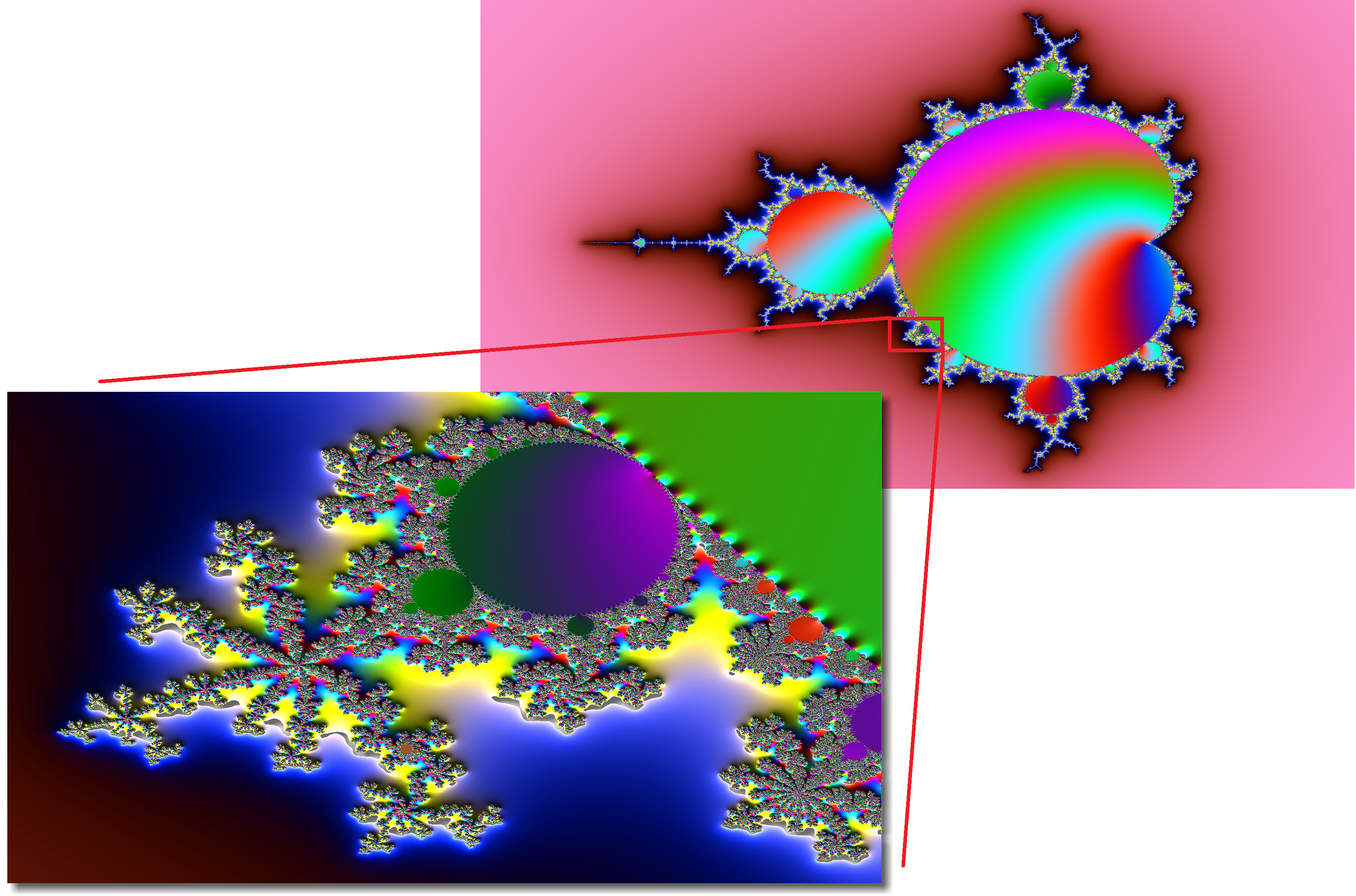
Figure 3. Detail of the Mandelbrot set illustrated as 3D object

3. Curves of the First Period

Curves of the m-th period are boundaries of areas called „bulbs“ which are described approximately only in present. In this paper, some of them are described analyticaly – curves of the first period, the boundary of the main hyperbolic component, internal and external bounds and also some curves of the second period.

In ^[1], we can read about the Mandelbrot set of the second degree: „It should be pointed out that the bulbs’ apparent circular shape is indeed only approximate.“ We proved ^[2] that the curve of the second period in this set is precise circle. The curves of the higher period cannot be precise circles because the Mandelbrot set is generated by nonlinear transforms. However, it is possible to obtain their analytical description on principle.

In the following text, we will analyse sets  for whichSets of points for which is

and

are callled a curve of the period. We denote . Curves of the first period are sets

3.1. The Boundary of the Main Hyperbolic Component

The main hyperbolic component  is the subset of for which the orbit does not diverge. It is bounded by . In case of ,

and equation of is possible to obtain from , i.e.

According to Banach fixed-point theorem, its points must satisfy the condition and for its boundary . These conditions lead to equation of the main hyperbolic components as

(see ^[2] for more information)

The subscript (1) means that is the curve of period one – if lies on this curve, then lies on the curve too. For the classic Mandelbrot set is and we have 

There is for and

By analogy

These curves are marked as pink in Figures 4,5,6.

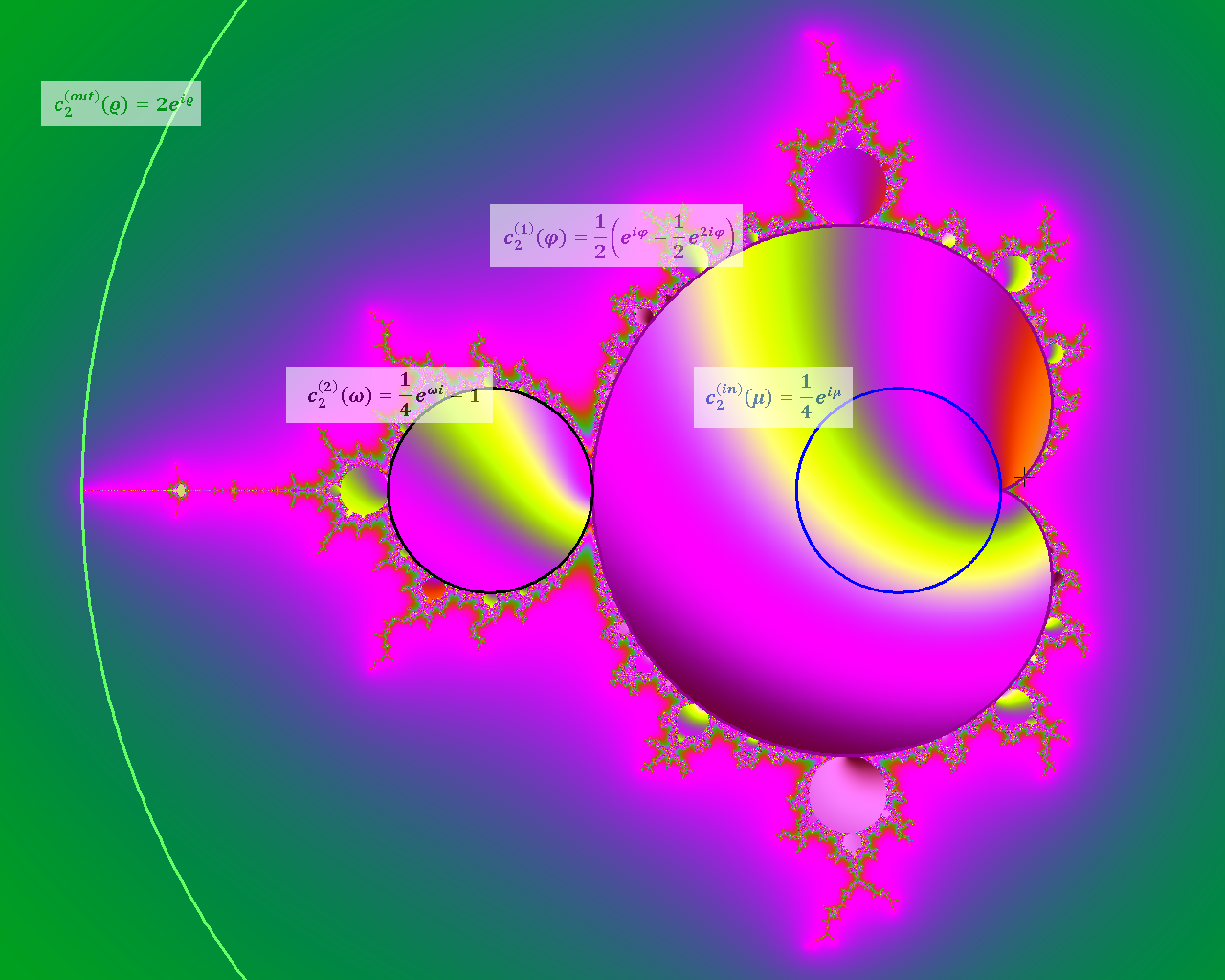
Figure 4. Curves of the first and second period for

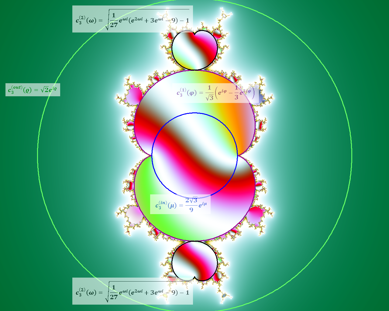
Figure 5. Curves of the first and second period for

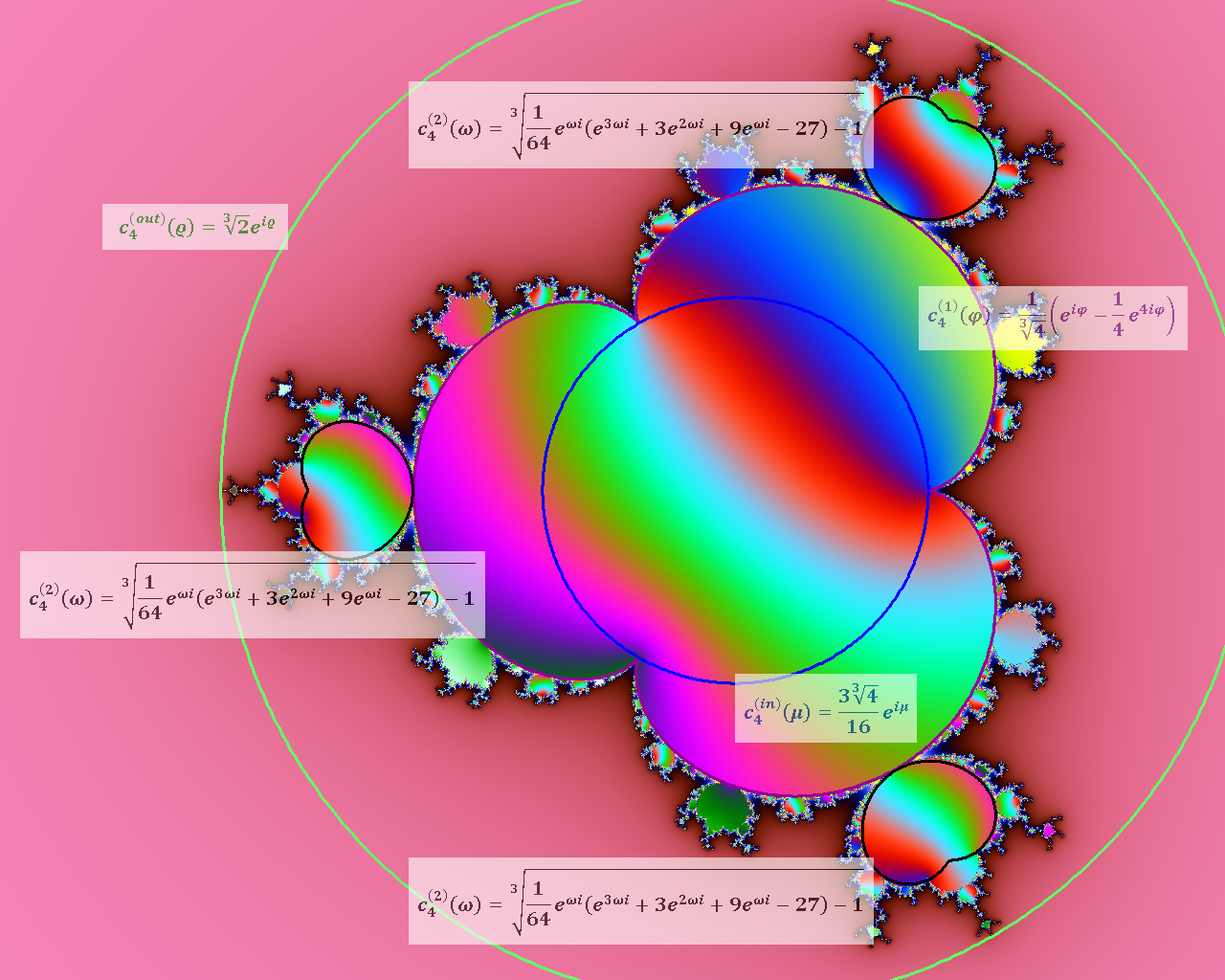
Figure 6. Curves of the first and second period for

It is important to note thatandand thereforeIt means that these curves converge into the unit circle.

3.2. Internal Bound

For speeding up rendering of the Mandelbrot set, it is possible to detect as internal points those belonging into the curve of period one. They lie on the circle with the centre and radius This condition gives

(see ^[2] for more information). These circles are marked as pink in Figures 2, 3, 4.

3.3. External Bound

Rendering of the Mandelbrot set is possible to accelerate also by external bound detection – the escape radius mentioned in section 2 does not have to be bigger than radius of the external bound. We can assume that outside the escape zone is already bigger than therefore

It means

(see ^[2] for more information). These circles are marked as pink in Figures 2, 3, 4.

4. Curves of the Second Period

Curves of the second period are sets

These curves are boundaries between convergence and divergence process

According to Banach fixed-point theorem, it must be

again.

4.1. Curves of the Second Period for  

We have to find roots of

that are not roots of

The calculations are already very technically dificult and are performed in ^[2].

The result is

This circle is marked as black in Figures 2, 3, 4.

4.2. Curves of the Second Period for

According to previous section: for , we have to find roots of

that are not roots of

The result is

For , we can obtain

5. Julia Sets

In case of the Mandelbrot set, iteration process

where is the constant start point and „lives“ in a rectangle. Therefore, there exists one and only one Mandelbrot set for given function .

On the other hand, Julia set arises as a result of iteration proces

where is constant and starting point „lives“ in a rectangle Therefore, there exist infinitely many Julia sets for each Mandelbrot set. This situation is illustrated in Figure 7.

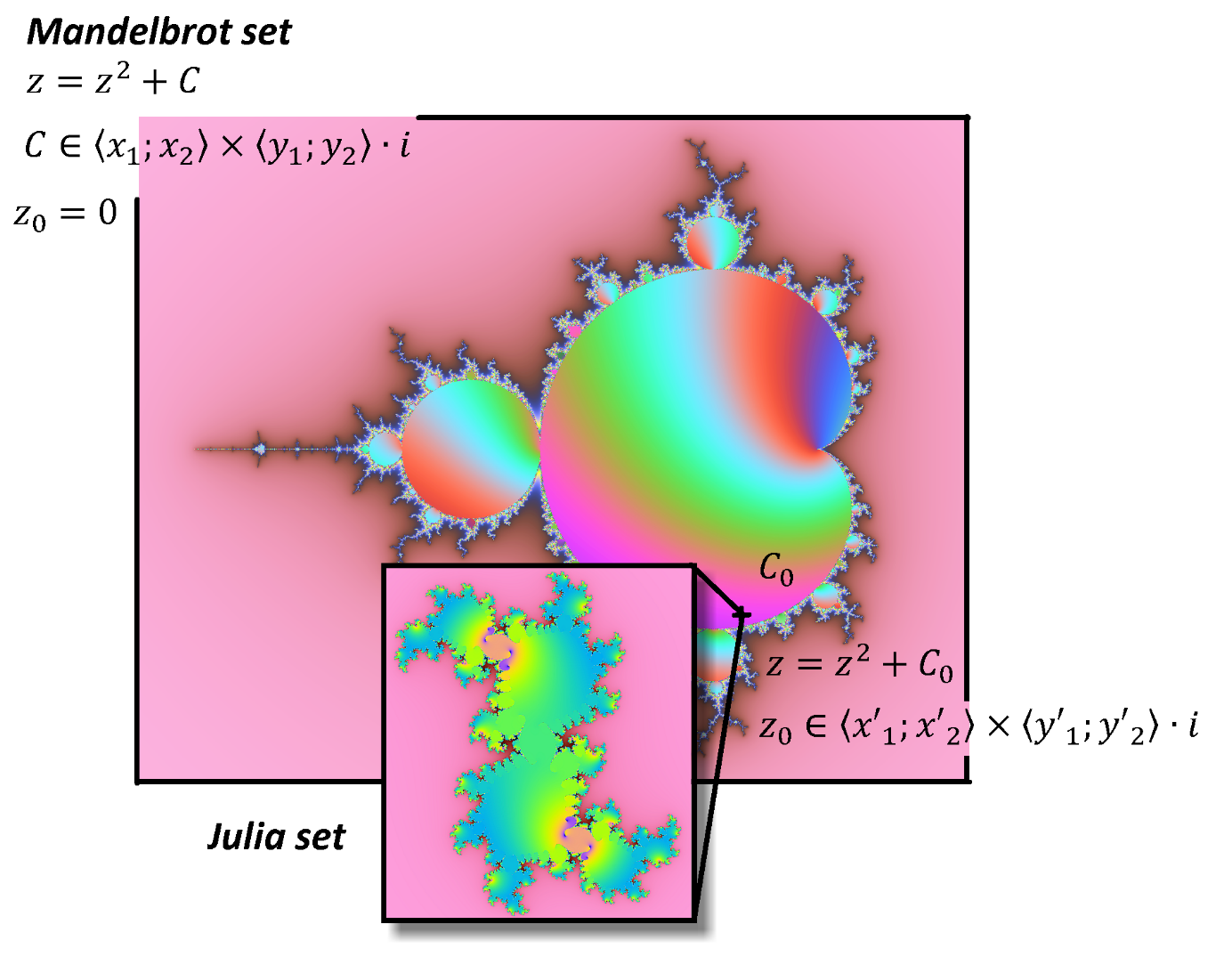
Figure 7. Mandelbrot set and its Julia sets.

6. Journey Around the Mandelbrot Set

If is placed inside Mandelbrot set, then Julia set is connected and it is disconnected in case of outside placement. The most interesting shapes of the Julia set can be found near the boundary of the Mandelbrot set, i. e. near its periodical curves. Complete video contains hundreds of thousands frames with Julia sets near the curve of the first and second period the classical Mandelbrot set (irregularly alternatively outside and inside). It runs a number of hours. Computing demandingness was approx. 80 days per (common) processor. For demonstration purposes, the video was shortened to less than seven minutes