1. Statistical terms

First we will organize the experimental data in a data table. This is a 2x2 matrix with the following format: the elements or subjects that are the focus of the study are located in rows, known as the units of analysis (UA₁, UA₂, ., UA_i), whereas the values of the random variables are located in columns (X₁, X₂, ., X_j). Therefore, a column vector (j) is a random sample, and a row vector (i) is an observation vector.

A random variable is an observable property. If it is quantitative then it can be continuous, that is, it is a measurable property or discrete when the property is countable. Random variables are classified according to the following criterion:

Quantitative: Discrete: 0, 1, 2,.; Continuous: 0.26, 1.81,. etc.

Qualitative: Ordinal or range (order): e.g. colors ordered by wavelength; Nominal (not order) : for example, colors blue, green, red etc.

On some occasions the researcher will use attributes (frequencies) are e.g. percentage of people in blood group A; or percentage of silicates in a given location. We will refer to the values of the variable X as observations, which we will represent as a sequence {x₁, x₂, . x_n}. In order to simplify the notation in this sequence, we refer with x₁ to the value of the variable in the first unit of analysis, x₂ to the value in the second unit of analysis, etc. The value of n is the sample size, i.e. the number of elements, objects or units of analysis in which the value of the random variable X has been obtained experimentally.

Descriptive statistics summarize the information contained in a sample into three classes of numerical values which are referred to as centralization, dispersion and shape measures.

 2. Univariate Descriptive Statistical Methods

In experimental work there are situations where a descriptive statistical analysis of a random variable X is required. The result of this analysis is a series of measures, known as centralization, dispersion and shape measures:

2.1. Centralization measures

Their purpose is to inform about the trend of data.

Sample size (n): This is not in itself a measure of centralization, although it is usually included in this group. It is the number of individuals, elements or objects that make up the sample. A large sample is one with more than 30 individuals (n>30), and a small sample is one with less than 30 (n<30).

Arithmetic mean ( ).- This is the average value of the observations. It is one of the most important measures of centralization:

Geometric mean (mg).- It is a mean value that is used with percentages, rates etc:

Harmonic mean (ma).- It is a very robust mean value to extreme values with utility in the calculation of the average of speeds, times, performances etc:

Quadratic mean (mc).- It is a mean value that is used in the calculation of the average of alternate currents, waves, gases, etc. removing the sign effects when some observations take negative values. It is also known as RMS or mean square value:

Median (Me).- If we order the values of the observations from lowest to highest the median is that observation that leaves 50% of the observations above and the other 50% below. It is known by other names such as 'quartile two', 'percentile 50'.

Mode (Mo).- It is the most frequent value in the observations.

Quantiles.- This is the application of what is known as elementary range theory, introduced by the statistician Kendall in 1940. If we order the values of the observations from lowest (MIN) to highest (MAX), we will have the following values or quantiles.

If we then divide the sample into four equal parts then Q1 (first quartile) will be the value that leaves 25% and 75% of the observations on the left and right, Q2 (second quartile) is the median (Me), and Q3 (third quartile) is the value that leaves 75% and 25% of the observations on the left and right.  Now, if we were to divide the sample into 100 equal parts then we would have percentiles. For example, P25, P50 and P75 correspond to Q1, Q2 and Q3 respectively.

2.2. Dispersion measures

These measures inform us of the variability or dispersion of the data, and therefore of the degree of representativity of the centralization measures. The lower the variability, the more representative the centralization measure obtained will be.

Range (r).- This is defined as the difference between the maximum and minimum values of the observations, i.e. Max(x)-min(x). It is used in quality control experiments.

Interquartile range (IQR).- It is a measure of variability defined from the quartile theory, being equal to Q3-Q1.

Mean Deviation (Dm).- A good indicator of dispersion defined as an average of the differences in absolute value of each observation with respect to the arithmetic mean:

Variance (s²).- It is the most important measure of dispersion in the experimental work, also known as mean square error. It is defined as an average of the squared differences of each observation with respect to the arithmetic mean:

Do not be mistaken with quasi-variance, an unbiased estimator's version of the variance (its mathematical expectation is the population variance, E[ ] =μ):

Standard deviation (s).- Is the square root of the variance (s²). In this way units are expressed linearly and not squared as with the variance.

Standard error: Since the sample mean is a random variable, as its value fluctuates from sample to sample, the standard error is the standard deviation of the arithmetic mean. It is used in statistical inference, although sometimes its value is included in descriptive statistics.

Pearson's coefficient of variation (CV): It is defined as the ratio of the standard deviation to the sample mean. It is usually multiplied by 100 allowing a comparison of the variability between any two variables:

2.3. Shape measurements

Its purpose is to measure the shape of the frequency distribution of the data. The shape of the distribution is quantified with two measurements:

Asymmetry (g₁ or 'skewness'): If the distribution is symmetric then g1 will be close to zero. Otherwise, when g₁>0 then a considerable number of data are concentrated in the high values of the distribution, being the distribution skewed to the right. If g₁<0 then the distribution will be biased towards the low values, i.e. towards the left. 

 Left-biased (g₁<0), unbiased (g₁=0) and right-biased (g₁>0) distributions 

Kurtosis (g₂ or 'kurtosis'): This is a measure of the sharpness of the data distribution. If g₂ is zero then the distribution is mesocurtic, if g₂>0 then it is called leptocurtic, and if g₂<0 then the distribution is termed platicurtic. In a leptocurtic distribution the variance s² is very low, while in a platicurtic distribution the variance s² is very high. Therefore, the variability has a mean value only when the distribution is mesocurtic.

Platicurtic (g₂<0), mesocurtic (g₂=0) and leptocurtic (g₂>0) distributions

3. Exploratory data analysis

In addition to the measures of centralization, dispersion and shape, the descriptive statistics use graphical methods. The most commonly used graphs in the experimental work are:

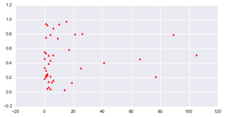
 Scatterplot.- Representation of the observations in which the X or x-axis represents the values of the data or observations, and the Y or y-axis is a dummy value obtained by simulating the "shaking" or "jitter" of the X axis, thus allowing a more comfortable visualization of the observations.

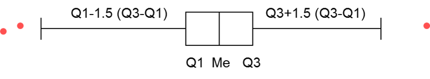
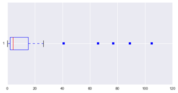
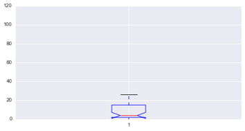
Box and whisker plot.- It is a graph currently widely used in experimental work. It was introduced by the statistician Tukey in 1977 and became popular with the widespread use of computers. It allows for analysis of (a) distribution symmetry, (b) identification of outliers and (c) comparison of batches of data.

Histogram.- One of the most popular graphs in descriptive statistics. It represents the distribution of frequencies in quantitative variables that are continuous. Not to be confused with bar charts used with discrete quantitative variables.

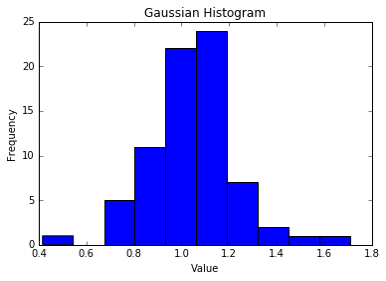
In a histogram the bars are rectangles representing intervals and have a height proportional to the frequency of each interval, once the data are grouped and organized in a table of classes and frequencies.

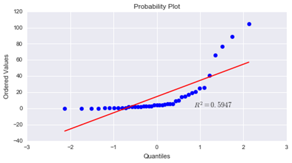
Normal Probability Chart.- Allows the evaluation of the normality of the variable under study by comparing the data with the normal distribution. That is, this graph evaluates whether or not the data come from a normal or Gaussian distribution in an empirical way, by fitting the points representing the experimental data to a straight line that would represent the normal distribution.

4. Python script description

Lines 33-60 calculate the measures of centralization, dispersion and shape. In addition, a test for normality of the data is included. First the script obtains the sample size, minimum, maximum and range values of the variable (lines 36-39). Next, the arithmetic mean (line 40), geometric mean (line 41), harmonic mean (line 42) and quadratic mean (line 43) are calculated. Mode is calculated in line 44, and quartiles Q1, Q2 and Q3 in lines 46-48. Other quartiles can be obtained by specifying the order np.percentile(data,_). The dispersion measures are obtained below. Variance, standard deviation, standard error of the mean, interquartile range and Pearson's deviation coefficient are calculated on lines 49-53. Finally, shape measurements are obtained, both asymmetry (line 55) and kurtosis (line 57). The script performs the D'Agostino and Pearson normality tests (line 59).

The most common graphic methods are performed with the code section displayed in the script between lines 61-93. Lines 63-77 show different versions of the order that allows to represent a box and whiskers plot with the experimental data. Line 65 shows the basic order for a box-and-whiskers plot. If a notch in the box is desired to plot a confidence interval for the median (Me) then the order is as shown on line 68. On line 74 the box-and-whisker plot is shown horizontally. Outliers are detected and plotted using the order on line 71. Finally, line 77 shows an order to obtain a box-and-whisker plot with longer whiskers.

A histogram is represented between lines 79-83. The number of classes and therefore of bars in the histogram can be set or an appropriate value estimated with the Sturges expression (line 82). Other characteristics of the histogram are specified with the order plt.hist(data,numBins,_,.,_). The code section below (lines 85-88) represents a scatter plot simulating with y_data the jitter of data and allowing the user to define some graphic characteristics in plt.scatter(data,y_data,_,.,_). Finally, between lines 90-93 a normal probability graph is displayed.

 1
 2
 3
 4
 5
 6
 7
 8
 9
10
11
12
13
14
15
16
17
18
19
20
21
22
23
24
25
26
27
28
29
30
31
32
33
34
35
36
37
38
39
40
41
42
43
44
45
46
47
48
49
50
51
52
53
54
55
56
57
58
59
60
61
62
63
64
65
66
67
68
69
70
71
72
73
74
75
76
77
78
79
80
81
82
83
84
85
86
87
88
89
90
91
92
93

############################################################
#                                                          #
#         Virtual Laboratory of Statistics in Python       #
#                                                          #
#       Univariate descriptive statistics  (01.01.2020)    #
#                                                          #                
#         Complutense University of Madrid, Spain          #
#                                                          #
#   THIS SCRIPT IS PROVIDED BY THE AUTHORS "AS IS" AND     #
#   CAN BE USED BY ANYONE FOR THE PURPOSES OF EDUCATION    #
#   AND RESEARCH.                                          #
#                                                          #
############################################################
import math
import numpy as np # importing numpy
import scipy.stats as s # importing scipy.stats
import statistics as ss # importing statistics  

# Embedded graphics
import matplotlib.pyplot as plt # importing matplotlib
import seaborn as sns # importing seaborn

import pylab

# Aesthetic parameters of seaborn
sns.set_palette("deep", desat=.6)
sns.set_context(rc={"figure.figsize": (8, 4)})

# Declare here the name of the data file
data=np.loadtxt('datafile.dat', skiprows=0)
print(data)

# Measures of centralization, dispersion and form
def quadratic_mean(num):
	return math.sqrt(sum(n*n for n in num)/len(num))
print('n = ',len(data))
print('Minimum = ',min(data))
print('Maximum = ',max(data))
print('Rank = ',max(data)-min(data))
print('Average = ',ss.mean(data))
print('Geometric mean= ',s.gmean(data))
print('Harmonic mean= ','s.hmean(data)')
print('Quadratic mean=',quadratic_mean(data))
print('Mode = ',s.mode(data))
print('Median = ',np.median(data))
print('Q1 = ',np.percentile(data,25))
print('Q2 = ',np.percentile(data,50))
print('Q3 = ',np.percentile(data,75))
print('Variance  =',ss.variance(data))
print('Standard deviation = ',ss.stdev(data))
print('Standard error of the mean  =',ss.stdev(data)/math.sqrt(len(data)))
print('Interquatile rank = ',np.percentile(data,75)-np.percentile(data,25))
print('Coefficient of variation = ',(ss.stdev(data)/ss.mean(data))*100)
print()
print('Skewness =',s.skewtest(data))
print()
print('Kurtosis = ',s.kurtosistest(data))
print()
print('Normality test (D’Agostino and Pearson’s ) = ',s.normaltest(data))
print()
# Descriptive statistics

# Box-and-Whisker plot
# basic plot
plt.boxplot(data,0,' ')
# notched plot
plt.figure()
plt.boxplot(data, 1,' ')
# change outliers symbols
plt.figure()
plt.boxplot(data, 1, 'gD')
# horizontal plot
plt.figure()
plt.boxplot(data, 0, 'rs', 0)
# whisker length change 
plt.figure()
plt.boxplot(data, 0, 'rs', 0, 0.75)

# Histogram
# histtype= normed=0 1 'bar' 'step', cumulative=0 1
plt.figure()
numBins = round(1+3.222*math.log10(len(data))) 
plt.hist(data,numBins,normed=0,color='green',alpha=0.8, histtype='bar', cumulative=0)
        
# Scatter plot 
y_data=[np.random.random() for x in range (0, len(data))]
plt.figure()
plt.scatter(data, y_data, color="red", marker="^")

# Normality probability plot 
plt.figure()
s.probplot(data, dist="norm", plot=pylab)
pylab.show()