Your browser does not fully support modern features. Please upgrade for a smoother experience.
Subjects:
Engineering, Electrical & Electronic
This article gives a brief overview of the Doherty technique. The Idea of the Doherty is the most straightforward technique for providing efficiency at the back-off, where no additional digital signal processing (DSP) nor additional circuits are required to be attached with the design.
Classical Doherty Power Amplifier Operation
In 1936, W.H. Doherty invented a new combiner designed for broadcasting stations using high power tube amplifiers [1]. A λ/4 transmission line was used as a combiner at the output of power amplifiers to achieve a linear output power. The classic DPA consists of two amplifiers known as the carrier (main) amplifier and the auxiliary (peaking) amplifier (Figure 1). A class AB amplifier used for the carrier amplifier whereas a class C amplifier is used for the peaking amplifier. The RF input signal is split between the two amplifiers, where the carrier amplifier is working all the time and should almost reach saturation at the back-off input power due to seeing a high impedance which causes a change in the load-line as shown in Figure 2. At the same power level, the auxiliary amplifier works only in the Doherty region and starts feeding current to the output till it becomes saturated at the peak region, where the two power amplifiers give their maximum designed output power.
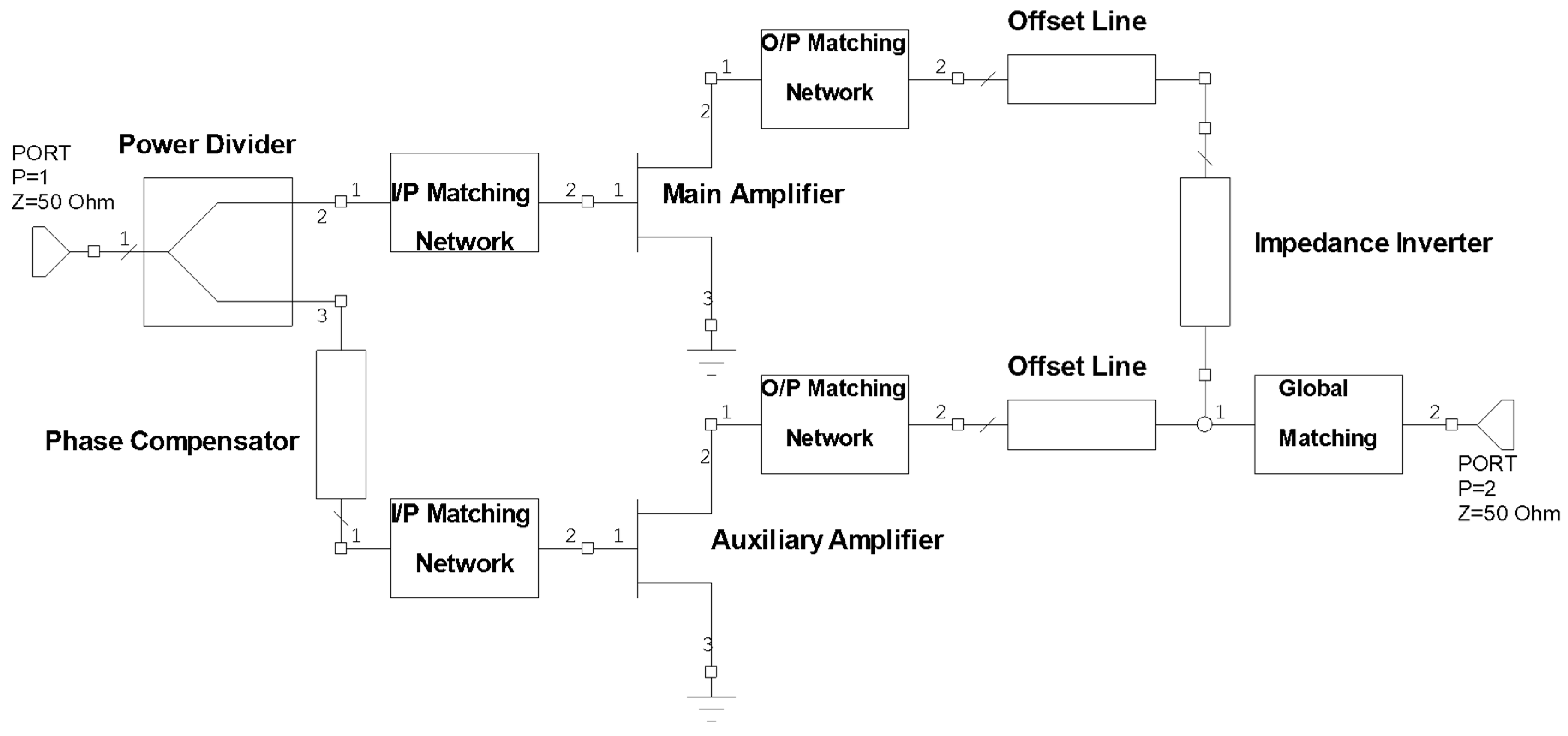
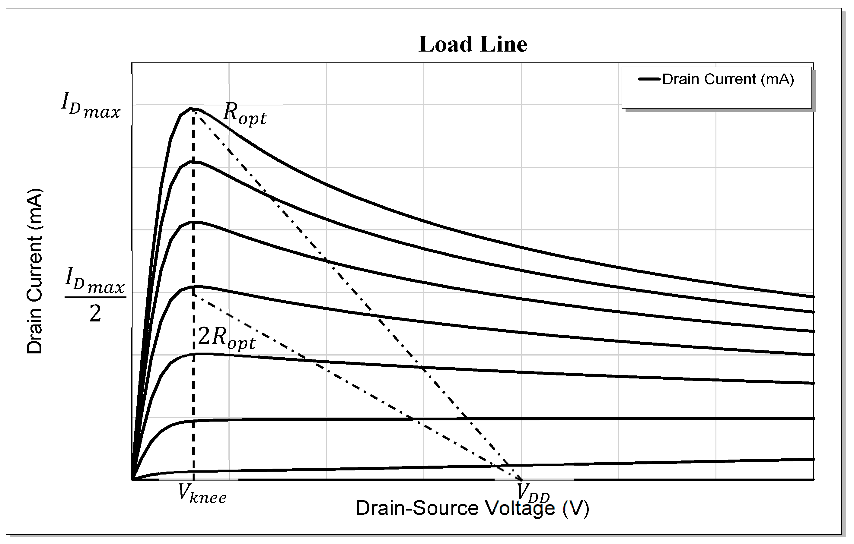
Figure 2. Main amplifier load line [2].
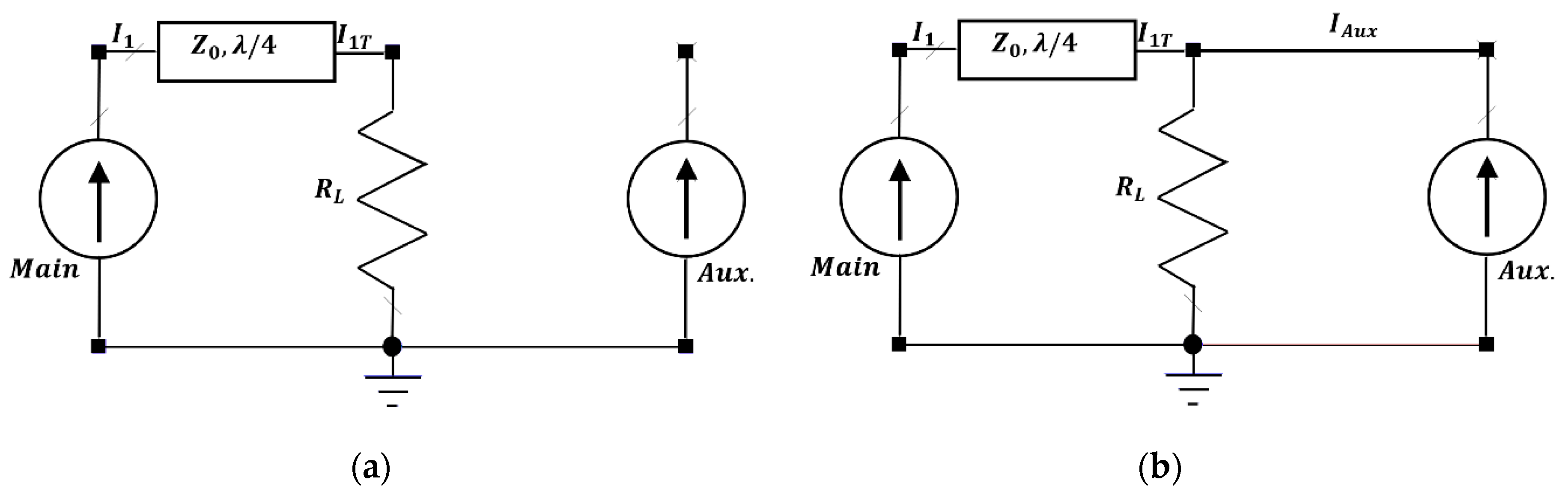
The idea of the Doherty amplifier depends on the so-called active load-pull technique [1]. Where the DPA operation can be divided into three regions:
The low RF input power region, where the signal level is not sufficient to turn the auxiliary amplifier on, in this case, the auxiliary amplifier can (theoretically) be represented as an open circuit as shown in Figure 3a. At the same time, the main amplifier is amplifying the input signal as an ordinary power amplifier, however, the load is seen by the main amplifier through the impedance inverter (λ/4 transmission line) and is increased because the characteristic impedance of the λ/4 transmission line is higher than the load impedance. In this case, the main amplifier will be almost saturated because its load line has changed, as illustrated in Figure 2. The impedance seen by the main amplifier depends on the following equation:
Z1=ZT2/RL
Where:
Figure 3. Doherty equivalent circuit diagram [2] (a) at low power region and (b) at medium and high-power region.
-
Z1: the impedance seen by the main amplifier
-
ZT: transmission line characteristic impedance
-
RL: the load
The second region (medium RF input power), where the auxiliary amplifier starts feeding current to the load and acts as an additional current source as illustrated in Figure 3b. As auxiliary amplifier current increases, the apparent load impedance seen by the impedance inverter at the summing node will increase, and hence, the impedance seen by the main amplifier will decrease, and the load line will move as shown in Figure 2. As a result, the output voltage of the main amplifier remains roughly constant, and the total current is increasing which increases the total output power. The following equations show the relationship between the impedance of each amplifier and the amplifiers’ currents:
where:
Z2=RL(1+I1T/IAux) (2)
Z1=ZT2RL/(1+IAux/I1T) (3)
-
Z2: the impedance seen by the auxiliary amplifier
-
I1T: the current after the λ/4 transmission line
-
IAux: current of the auxiliary amplifier
Finally, the high-power region, where both amplifiers work at their maximum output current and the impedance seen by each amplifier is controlled also by Equations (2) and (3). The load modulation occurs in the last two regions, where the benefit of Doherty structure is clear.
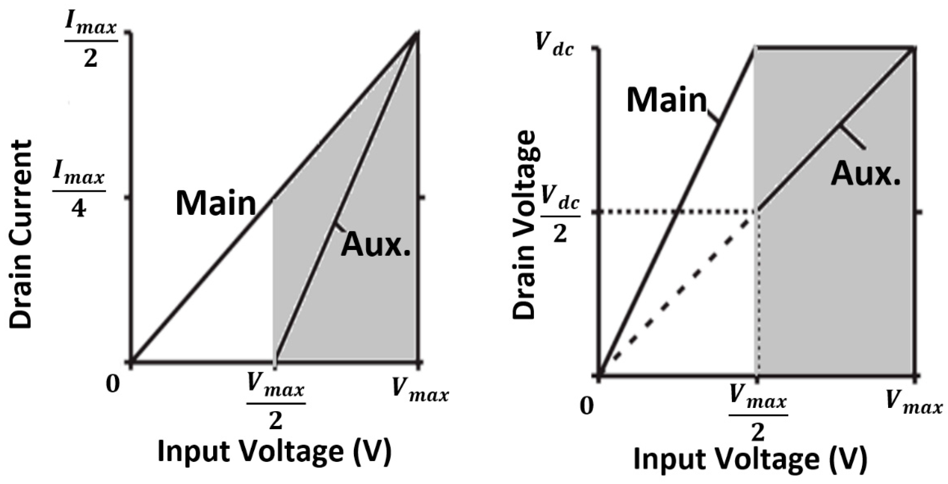
The main and the auxiliary current and voltage behavior is shown in Figure 4. The auxiliary amplifier starts contributing its current near the OBO point, whereas the main amplifier voltage remains roughly constant after the OBO point but its current increases.
Figure 4. Voltage and current behavior of Doherty amplifier [3].
- Doherty, W.H. A new high-efficiency power amplifier for modulated waves. Bell Syst. Tech. J. 1936, 15, 469–475.
- Abdulkhaleq, A.M.; Yahya, M.A.; McEwan, N.; Rayit, A.; Abd-Alhameed, R.A.; Ojaroudi Parchin, N.; Al-Yasir, Y.I.A.; Noras, J. Recent Developments of Dual-Band Doherty Power Amplifiers for Upcoming Mobile Communications Systems. Electronics 2019, 8, 638
- Barakat, A.; Thian, M.; Fusco, V.; Bulja, S.; Guan, L. Toward a More Generalized Doherty Power Amplifier Design for Broadband Operation. IEEE Trans. Microw. Theory Tech. 2017, 65, 846–859.