Your browser does not fully support modern features. Please upgrade for a smoother experience.
Please note this is an old version of this entry, which may differ significantly from the current revision.
Image segmentation, which has become a research hotspot in the field of image processing and computer vision, refers to the process of dividing an image into meaningful and non-overlapping regions, and it is an essential step in natural scene understanding.
- image segmentation
- co-segmentation
- semantic segmentation
- deep learning
- image processing
1. Introduction
Image segmentation is one of the most popular research fields in computer vision, and forms the basis of pattern recognition and image understanding. The development of image segmentation techniques is closely related to many disciplines and fields, e.g., autonomous vehicles [1], intelligent medical technology [2,3], image search engines [4], industrial inspection, and augmented reality.
Image segmentation divides images into regions with different features and extracts the regions of interest (ROIs). These regions, according to human visual perception, are meaningful and non-overlapping. There are two difficulties in image segmentation: (1) how to define “meaningful regions”, as the uncertainty of visual perception and the diversity of human comprehension lead to a lack of a clear definition of the objects, it makes image segmentation an ill-posed problem; and (2) how to effectively represent the objects in an image. Digital images are made up of pixels, that can be grouped together to make up larger sets based on their color, texture, and other information. These are referred to as “pixel sets” or “superpixels”. These low-level features reflect the local attributes of the image, but it is difficult to obtain global information (e.g., shape and position) through these local attributes.
2. Classic Segmentation Methods
The classic segmentation algorithms were proposed for grayscale images, which mainly consider gray-level similarity in the same region and gray-level discontinuity in different regions. In general, region division is based on gray-level similarity, and edge detection is based on gray-level discontinuity. Color image segmentation involves using the similarity between pixels to segment the image into different regions or superpixels, and then merging these superpixels.
2.1. Edge Detection
The positions where the gray level changes sharply in an image are generally the boundaries of different regions. The task of edge detection is to identify the points on these boundaries. Edge detection is one of the earliest segmentation methods and is also called the parallel boundary technique. The derivative or differential of the gray level is used to identify the obvious changes at the boundary. In practice, the derivative of the digital image is obtained by using the difference approximation for the differential. Examples of edge detection results are represented in Figure 2.
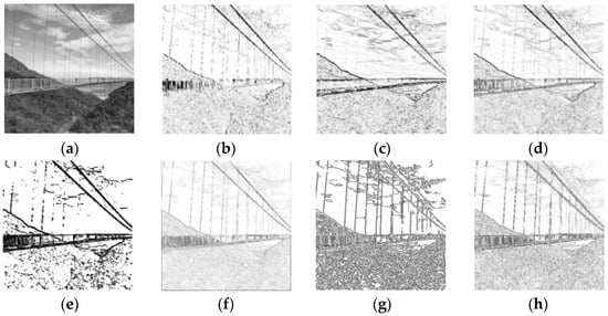
Figure 2. Edge detection results of different differential operators. (a) Original (b) SobelX (c) SobelY (d) Sobel (e) Kirsch (f) Roberts (g) Canny and (h) Laplacian.
These operators are sensitive to noise and are only suitable for images with low noise and complexity. The Canny operator performs best among the operators shown in Figure 2. It has strong denoising ability, and also processes the segmentation of lines well with continuity, fineness, and straightness. However, the Canny operator is more complex and takes longer to execute. In the actual industrial production, a thresholding gradient is usually used in the case of high real-time requirement. On the contrary, the more advanced Canny operator is selected in the case of high quality requirement.
Although differential operators can locate the boundaries of different regions efficiently, the closure and continuity of the boundaries cannot be guaranteed due to numerous discontinuous points and lines in the high-detail regions. Therefore, it is necessary to smooth the image before using a differential operator to detect edges.
Another edge detection method is the serial boundary technique, that concatenates points of edges to form a closed boundary. Serial boundary techniques mainly include graph-searching algorithms and dynamic programming algorithms. In graph-searching algorithms, the points on the edges are represented by a graph structure, and the path with the minimum cost is searched in the graph to determine the closed boundaries, which is always computationally intensive. The dynamic programming algorithm utilizes heuristic rules to reduce the search computation.
The active contours method approximates the actual contours of the objects by matching the closed curve (i.e., the initial contours based on gradient) with the local features of the image, and finds the closed curve with the minimum energy by minimizing the energy function to achieve image segmentation. The method is sensitive to the location of the initial contour, so the initialization must be close to the target contour. Moreover, its non-convexity easily leads to the local minimum, so it is difficult to converge to the concave boundary. Lankton and Tannenbaum [9] proposed a framework that considers the local segmentation energy to evolve contours, that could produce the initial localization according to the locally based global active contour energy and effectively segment objects with heterogeneous feature profiles.
2.2. Region Division
The region division strategy includes serial region division and parallel region division. Thresholding is a typical parallel region division algorithm. The threshold is generally defined by the trough value in a gray histogram with some processing to make the troughs in the histogram deeper or to convert the troughs into peaks. The optimal grayscale threshold can be determined by the zeroth-order or first-order cumulant moment of the gray histogram to maximize the discriminability of the different categories.
The serial region technique involves dividing the region segmentation task into multiple steps to be performed sequentially, and the representative steps are region growing and region merging.
Region growing involves taking multiple seeds (single pixels or regions) as initiation points and combining the pixels with the same or similar features in the seed neighborhoods in the regions where the seed is located, according to a predefined growth rule until no more pixels can be merged. The principle of region merging is similar to the region growing, except that region merging measures the similarity by judging whether the difference between the average gray value of the pixels in the region obtained in the previous step and the gray value of its adjacent pixels is less than the given threshold K. Region merging can be used to solve the problem of hard noise loss and object occlusion, and has a good effect on controlling the segmentation scale and processing unconventional data; however, its computational cost is high, and the stopping rule is difficult to affirm.
2.3. Graph Theory
The image segmentation method based on graph theory maps an image to a graph, that represents pixels or regions as vertices of the graph, and represents the similarity between vertices as weights of edges. Image segmentation, based on graph theory, is regarded as the division of vertices in the graph, analyzing the weighted graph with the principle and method based on graph theory, and obtaining optimal segmentation with the global optimization of the graph (e.g., the min-cut).
Graph-based region merging uses different metrics to obtain optimal global grouping instead of using fixed merging rules in clustering. Felzenszwalb et al. [11] used the minimum spanning tree (MST) to merge pixels after the image was represented as a graph.
Image segmentation based on MRF (Markov random field) introduces probabilistic graphical models (PGMs) into the region division to represent the randomness of the lower-level features in the images. It maps the image to an undigraph, where each vertex in the graph represents the feature at the corresponding location in the image, and each edge represents the relationship between two vertices. According to the Markov property of the graph, the feature of each point is only related to its adjacent features.
2.4. Clustering Method
K-means clustering is a special thresholding segmentation algorithm that is proposed based on the Lloyd algorithm. The algorithm operates as follows: (i) initialize K points as clustering centers; (ii) calculate the distance between each point i in the image and K cluster centers, and select the minimum distance as the classification ki; (iii) average the points of each category (the centroid) and move the cluster center to the centroid; and (iv) repeat steps (ii) and (iii) until algorithm convergence. Simply put, K-means is an iteration process for computing the cluster centers. The K-means has noise robustness and quick convergence, but it is not conducive to processing nonadjacent regions, and it can only converge to the local optimum solution instead of the global optimum solution.
Spectral clustering is a common clustering method based on graph theory, that divides the weighted graph and creates subgraphs with low coupling and high cohesion. Achanta et al. [15] proposed a simple linear iterative clustering (SLIC) algorithm that used K-means to generate superpixels; its segmentation results are shown in Figure 3. SLIC can be applied to 3D supervoxel generation.
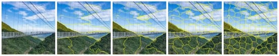
Figure 3. SLIC segmentation results (number of superpixels: 10, 20, 50, and 100).
2.5. Random Walks
Random walks is a segmentation algorithm based on graph theory, that is commonly used in image segmentation, image denoising [17,18], and image matching [19]. By assigning labels to adjacent pixels in accordance with predefined rules, pixels with the same label can be represented together to distinguish different objects.
3. Co-Segmentation Methods
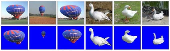
The classic segmentation methods usually focus on the feature extraction of a single image, which makes it difficult to obtain the high-level semantic information of the image. In 2006, Rother et al. [24] proposed the concept of collaborative segmentation for the first time. Collaborative segmentation, or co-segmentation for short, involves extracting the common foreground regions from multiple images with no human intervention, to obtain prior knowledge. Figure 4 shows a set of examples of co-segmentation results.
Figure 4. Two examples of co-segmentation results.
3.1. MRF-Based Co-Segmentation
Rother et al. [24] extended the MRF segmentation and utilized prior knowledge to solve the ill-posed problems in multiple image segmentation. First, they segmented the foreground of the seed image, and assumed that the foreground objects of a set of images are similar; then, they built the energy function according to the consistency of the MRF probability distribution and the global constraint of the foreground feature similarity; finally, they estimated whether each pixel belongs to the foreground or background by minimizing the energy function to achieve the segmentation of the foreground and background.
3.2. Co-Segmentation Based on Random Walks
Collins et al. [33] extended the random walks model to solve the co-segmentation problem, further utilized the quasiconvexity to optimize the segmentation algorithm, and provided a professional CUDA library to calculate the linear operation of the image sparse features. Fabijanska et al. [34] proposed an optimized random walks algorithm for 3D voxel image segmentation, using a supervoxel instead of a single voxel, which greatly saved computing time and memory resources.
3.3. Co-Segmentation Based on Active Contours
Meng et al. [38] extended the active contour method to co-segmentation, constructed an energy function based on foreground consistency between images and background inconsistency within each image, and solved the energy function minimization by level set. Zhang et al. [39] proposed a deformable co-segmentation algorithm which transformed the prior heuristic information of brain anatomy contained in multiple images into the constraints controlling the brain MRI segmentation, and acquired the minimum energy function by level set, solving the problem of brain MRI image segmentation.
3.4. Clustering-Based Co-Segmentation
Clustering-based co-segmentation is an extension of the clustering segmentation of a single image. Joulin et al. [41] proposed a co-segmentation method based on spectral clustering and discriminative clustering. They used spectral clustering to segment a single image based on local spatial information, and then used discriminative clustering to propagate the segmentation results in a set of images to achieve co-segmentation. Kim et al. [42] divided the image into superpixels, used a weighted graph to describe the relevance of superpixels, converted the weighted graph into an affinity matrix to describe the relation of the intra-image, and then adopted spectral clustering to achieve co-segmentation.
3.5. Co-Segmentation Based on Graph Theory
Co-segmentation based on graph theory partitions an image into a digraph.
In contrast to the digraph mentioned earlier, Meng et al. [44] divided each image into several local regions based on the object detection, and then used these local regions as nodes to construct a digraph instead of using superpixels or pixels as nodes. Nodes are connected by directed edges, and the weight of the edges represents the local region similarity and saliency map between the two objects. Thereupon, the image co-segmentation problem was converted into the problem of finding the shortest path on the digraph.
3.6. Co-Segmentation Based on Thermal Diffusion
Thermal diffusion image segmentation maximizes the temperature of the system by changing the location of the heat source, and its goal is to find the optimal location of the heat source to achieve the best segmentation effect. Anisotropic diffusion is a nonlinear filter that can not only reduce the Gaussian noise but also preserve image edges. It is often used in image processing to reduce noise while enhancing image details. Kim et al. [46] proposed a method called CoSand, that adopted temperature maximization modeling on anisotropic diffusion, where k heat sources maximize the temperature corresponding to the segmentation of k-categories; they achieved large-scale multicategory co-segmentation by maximizing the segmentation confidence of each pixel in the image.
3.7. Object-Based Co-Segmentation
Alexe et al. [48] proposed an object-based measurement method to quantify the possibility that an image window contains objects of any category. The probability of whether it is an object in each sampling window was calculated in advance, and the highest scoring window was used as the feature calibration for each category of objects according to the Bayesian theory. The method could distinguish between objects with clear spatial boundaries, e.g., telephones, as well as amorphous background elements, e.g., grass, that greatly reduced the number of specified category object detection windows.
4. Semantic Segmentation Based on Deep Learning
With the continuous development of image acquisition equipment, there has been a great increase in the complexity of image details and the difference in objects (e.g., scale, posture). Low-level features (e.g., color, brightness, and texture) are difficult to obtain good segmentation results from, and feature extraction methods based on manual or heuristic rules cannot meet the complex needs of current image segmentation, that puts forward the higher generalization ability of image segmentation models.
Semantic texton forests [51] and random forest [52] methods were generally used to construct semantic segmentation classifiers before deep learning was applied to the field of image segmentation. For the past few years, deep learning algorithms have been increasingly applied to segmentation tasks, and the segmentation effect and performance have been significantly improved. The original approach divides the image into small patches to train a neural network and then classifies the pixels. This patch classification algorithm [53] has been adopted because the fully connected layers of the neural network require fixed-size images.
4.1. Encoder–Decoder Architecture
Encoder–decoder architecture is based on FCNs. Prior to FCNs, convolutional neural networks (CNNs) achieved good effects in image classification, e.g., LeNet-5 [55], AlexNet [56], and VGG [57], whose output layers are the categories of images. However, semantic segmentation needs to map the high-level features back to the original image size after obtaining high-level semantic information. This requires an encoder–decoder architecture.
In the encoder stage, convolution and pooling operations are mainly performed to extract high-dimensional features containing semantic information. The convolution operation involves performing the multiplication and summing of the image-specific region with different convolution kernels pixel-for-pixel, and then transforming the activation function to obtain a feature map. The pooling operation involves sampling within a certain region (the pooling window), and then using a certain sampling statistic as the representative feature of the region. The backbone blocks commonly used in segmentation network encoders are VGG, Inception [58,59], and ResNet [60].
4.2. Skip Connections
Skip connections or shortcut connections were developed to improve rough pixel positioning. With deep neural network training, the performance decreases as the depth increases, which is a degradation problem. To ameliorate this problem, different skip connection structures have been proposed in ResNet and DenseNet [63]. In contrast, U-Net [64] proposed a new long skip connection. U-Net makes jump connections and cascades of features from layers in the encoder to the corresponding layers in the decoder to obtain the fine-grained details of images.
4.3. Dilated Convolution
Dilated convolution, also known as atrous convolution, is constructed by inserting holes into the convolution kernel to expand the receptive field and reduce the computation during down-sampling. In FCN, the max-pooling layers are replaced by dilated convolution to maintain the receiving field of the corresponding layer and the high resolution of the feature map.
The DeepLab series [65,66,67,68] are classic models in the field of semantic segmentation. Prior to putting forward DeepLab V1, the semantic segmentation results were usually rough due to the transfer invariance lost in the pooling process, and the probabilistic relationship between labels not used for prediction. To ameliorate these problems, DeepLab V1 [65] uses dilated convolution to solve the problem of resolution reduction during up-sampling, and uses fully connected conditional random fields (fully connected CRFs) to optimize the post-processing of segmented images to obtain objects at multi-scales and context information.
4.4. Multiscale Feature Extraction
Spatial pyramid pooling (SPP) was proposed to solve the problem of the CNNs requiring fixed-size input images. He et al. [71] developed the SPP-net and verified its effectiveness in semantic segmentation and object detection. To make the most of image context information, Zhao et al. [72] developed PSPNet with a pyramid pooling module (PPM). Using ResNet as the backbone network, the PSPNet utilized PPM to extract and aggregate different subregion features at different scales, that were then up-sampled and concatenated to form the feature map, that carried both local and global context information. It is particularly worth noting that the number of pyramid layers and the size of each layer are variable, that depend on the size of the feature map input to the PPM.
4.5. Attention Mechanisms
To represent the dependency between different regions in an image, especially the long-distance regions, and obtain their semantic relevance, some methods commonly used in the field of natural language processing (NLP) have been applied to computer vision, that have made good achievements in semantic segmentation. The attention mechanism was first put forward in the computer vision field in 2014. The Google Mind team [78] adopted the recurrent neural network (RNN) model to apply attention mechanisms to image classification, making attention mechanisms gradually popular in image processing tasks.
RNN can model the short-term dependence between pixels, connect pixels, and process them sequentially, which establishes a global context relationship.
LSTM (long short-term memory) adds a new function to record long-term memory, that can represent long-distance dependence. Byeon et al. [81] used LSTM to achieve pixel-for-pixel segmentation of scene images, which proved that image texture information and spatial model parameters could be learned in a 2D LSTM model.
Self-attention mechanisms are mostly used in the encoder network to represent the correlation between different regions (pixels) or different channels of the feature maps. It computes a weighted sum of pairwise affinities across all positions of a single sample to update the feature at each position. Self-attention mechanisms have produced many influential achievements in image segmentation, e.g., PSANet [85], DANet [86], APCNet [75], CARAFE [87], and CARAFE++ [88].
This entry is adapted from the peer-reviewed paper 10.3390/electronics12051199
This entry is offline, you can click here to edit this entry!