Your browser does not fully support modern features. Please upgrade for a smoother experience.
Please note this is an old version of this entry, which may differ significantly from the current revision.
Subjects:
Engineering, Electrical & Electronic
The smart grid concept is introduced to accelerate operational efficiency and enhance the reliability and sustainability of the power supply. The load forecasting technique involves estimating future loads using historical and present data. In a smart grid, the forecasting of loads is done by considering the power consumption by users and the power produced by all types of generations (renewable and non-renewable) with the help of smart energy meters.
- smart grid
- smart sensors
- load forecasting (LF)
- machine learning
- parametric methods
- non-parametric methods
1. Introduction
Globally, the demand of electricity is increasing day by day. The growing use of electricity has prompted multiple agencies to implement a variety of strategies for maximizing its efficiency like: efficient use of fuels and raw materials during generation, input of organic and inorganic wastes into boilers, reducing auxiliary power consumption, the intelligent switching of domestic loads in the distribution network, continuously monitoring the reduction of power loss in transmission and distribution systems, utilizing energy-efficient equipment, educating society about better load optimization, etc. Based on the above discussion, one step would be to predict the future load for each type of consumer (domestic, commercial, and industrial). For this reason, researchers are concentrating more on load forecasting. The load forecasting technique involves estimating future loads using historical and present data. In smart grid, the forecasting of loads is done by considering the power consumption by users and the power produced by all types of generations (renewable and non-renewable) with the help of smart energy meters, as shown in Figure 1. Moreover, load forecasting is becoming more difficult these days due to two reasons: firstly, due to the privatization and deregulation of distribution companies/power industries in many countries, the consumer is free to select any electricity provider of their choice among the other providers [1,2,3]. Hence, a consumer will always choose a supplier whose cost is beneficial to them in their case. In this scenario, forecasters face challenges. Secondly, due to the availability of renewable sources like solar and wind power, their uncertainty has been increased due to their inconsistent behavior [1,2,3,4,5,6,7,8,9]. In [4,5,6,7,8,9], the authors stated that due to the inherent variability of renewable resources like solar and wind energy, there is uncertainty in the consumer demand. A rapid penetration of renewable energy sources with high variability and uncertainty presents new challenges to the operation of power systems. Due to random fluctuations in weather condition, the RES may suffer from uncontrollable generation. Energy produced by user-owned generators like PV and wind power is measured with dedicated meters. Two levels of metering are used in these generation plants, one installed at the point of common coupling, which is located at the power control center end (PCC) for energy exchange, and the other installed at the user-owned generator end for measuring the actual power produced. As a result, the data regarding the actual load could be reconstructed as a net of power data, and these data could then be considered for load forecasting. In contrast to this, Kaur et al. [10] presented a load forecasting scheme based on net power. Here, the forecasting of solar or wind energy is done separately, and the forecasting of load is done separately. Then, solar/wind forecasting and load forecasting are integrated to provide a net load forecast. It should be noted that inadequate forecasting may result in an unpredicted increase in operating cost due to the continuous operation of heavily loaded generators and an inappropriate capacity of reserve allocation [11].
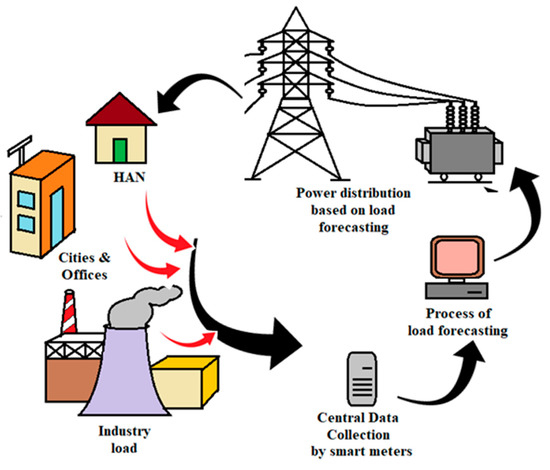
Figure 1. Process of load forecasting in a smart grid.
2. Load Forecasting Category
Based on the time horizon, load forecasting in smart grid is classified into four categories. A description of each category can be found in Table 1.
Table 1. Load forecasting categories based on time horizon and applications.
| Category | Time Horizon | Weather Historical Data | Application | ||||
|---|---|---|---|---|---|---|---|
| Load Scheduling |
Load Flow Planning | Preventive Maintenance | Fuel Procurement Planning | Future Unit Expansion | |||
| VSTLF | Few mins to 1 h | No |  |
||||
| STLF | 1 h to days | Yes | |
||||
| MTLF | Few days to months | Yes | |
|
|||
| LTLF | >1 year | Yes | |
||||
2.1. Very Short-Term Load Forecasting (VSTLF)
In VSTLF, the load forecasting is performed for a very short duration which ranges from a few minutes to an hour [17,18,19,20,21,22,23]. VSTLF is used for the real-time scheduling of generation, load frequency control, and resource dispatch [17,22]. It also plays an important role in auction-based electricity markets [20]. Various power networks, including those of Great Britain, China, and ISO New England, use VSTLF [17,18,22].
2.2. Short-Term Load Forecasting (STLF)
In STLF, load forecasting is performed for a short duration, i.e., from an hour to few days [13,24,25,26]. STLF can play an important role in any organization, planning for the proper load flow and avoiding the condition of overloading in the system [27]. In large-scale applications, such as where one country or group of nations (like the European Union) share a single power grid, the STLF plays a crucial role in making decisions regarding load [28].
2.3. Medium-Term Load Forecasting (MTLF)
In this type, the forecasting is performed for a duration ranging from a few days to several months to a year, as defined in [24,29,30]. MTLF is useful for planning and scheduling the preventive maintenance of unit and allows the organization to plan for raw material and fuel procurement [27].
2.4. Long-Term Load Forecasting (LTLF)
In LTLF, forecasting is performed for a duration ranging from one year to several years. Long-term forecasting accuracy is highly dependent on other variables such as weather [24,31]. LTLF is used for any organization to plan for their unit expansion or any major equipment installation [15].
3. Key Performance Indicators (KPI) for Load Forecasting
Whenever there is an error in load forecasting, the electricity suppliers may have to endure high production costs for electricity and sometimes they may be forced to go out of business because of a system failure causing a blackout [32]. It is, therefore, necessary to forecast accurately to enhance the system’s reliability and ensure uninterrupted power production. Hence, to measure the accuracy of any load forecasting technique, various KPIs are identified, which are describes as follows [20,26]:
3.1. Mean Absolute Error (MAE)
This can be calculated by the mean of the absolute error, where error (et) may be defined as the difference of the forecasted value (ft) and the actual value (at), as seen in Equation (1). Since the calculated error may be a negative or a positive value, the absolute value is used for MAE, which can be calculated using Equation (2).
3.2. Mean Absolute Percentage Error (MAPE)
MAPE is the division of the sum of all individual absolute errors and the actual value. It is calculated by the formula seen in Equation (3).
3.3. Root Mean Square Error (RMSE)
For RMSE, first we need to calculate the mean squared error (MSE) using Equation (4). Then, the square root of the average squared error is estimated using Equation (5).
3.4. Root Relative Squared Error (RRSE)
RRSE is the total squared error relative to the errors which have been formed if the forecasting is the average of the absolute value [14]. In other terms, RRSE is the square root of the ratio of the sum of the squared error of the forecasted and actual values to sum of the squared error of the average value and actual value. The relation for RRSE is seen in Equation (6).
where is the average of the actual value.
3.5. Coefficient of Variation (CV)
Coefficient of variation is calculated by the ratio of the predicted error standard deviation to the mean of the actual value or, in short, it is the ratio of RMSE to the mean of the actual value (a¯t), as mentioned in Equations (7) and (8) [33].
4. Data Pre-Processing
In smart grid, the data are collected through smart meters installed at the consumer’s end, the distribution transformer end, the substation end, and the generation end. In accordance with the method used, different datasets are collected from smart meters over different time horizons (e.g., 15 min, 30 min, 1 h, 1 day, 1 month, and 1 year). However, when compiling the dataset, it is not necessary to obtain the complete data at each time point; sometimes there may be missing data in the dataset for any duration, sometimes there may be outliers which overshoot or undershoot the dataset, and sometimes there is huge elimination of the dataset due to technical reasons. Therefore, in order to pre-process the dataset, various methods such as elimination, interpolation, and noise extraction are employed (Figure 2).
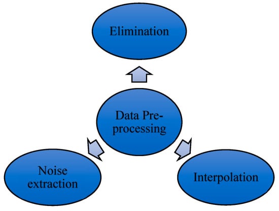
Figure 2. Data pre-processing methods.
4.1. Elimination
In the elimination method, the user has huge unrecorded/missing data which are excluded from load forecasting considerations [32]. Furthermore, if there is a big loss of data in the dataset, then this loss of data is also eliminated from the dataset as well. If this is not conducted, then it may affect the accuracy of forecasting.
4.2. Interpolation
During the process of collecting the data, there are certain times when we may not acquire the values in between two data. Therefore, the missing data are interpolated over these single missing values. Hence, interpolation is a process of filling in missing data by interpolating the previous and next values of the missing value [34,35]. Equation (9) represents the formula of interpolation.
where cn is the missing value, cn−1 is previous value to cn, and cn+1 is next value to cn. dn, dn−1, and dn+1 are the time of data with respect to cn,cn−1, and cn+1.
4.3. Noise Extraction
Since the data are exported from the server, they contain a wide variety of noise which needs to be removed before the load forecasting model can be constructed, to ensure accurate predictions. The noises are in the terms of negative load values and some random codes [36].
4.4. Imputation
Imputation methods are most commonly used in statistics in order to overcome the problem of missing data with a substitute value [37]. In general, there are two types: single and multiple imputations. In single imputation, each missing value is replaced by a single value. In contrast, in multiple imputation, certain rules are applied to substitute the missing value [38]. Moreover, the method of imputation can further be classified as maximum likelihood imputation (MLI) methods and machine learning (ML)-based methods [39]. The MLI contains expected maximization, multiple imputation, and Bayesian principal component analysis. Additionally, the ML-based methods involve imputation with K-nearest neighbor (KNN), weighted imputation with KNN, K-means clustering imputation, imputation with fuzzy K-means clustering, SVM imputation, singular value decomposition imputation, local least square imputation, etc. [39].
5. Process of Load Forecasting
Generally, the process of forecasting load is the same for all the categories, as well as all the methods. The process of load forecasting has different steps, as shown in Figure 3.
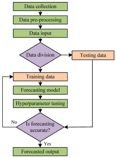
Figure 3. Process flow diagram of load forecasting.
5.1. Data Collection
In order to forecast load, the first requirement is to collect the data. The data can be collected in various ways for load forecasting, such as manually taking the data at the customer end or at the distribution transformer end, collecting recorded data through smart meters, collecting data from the main server, and sometimes taking data that are already recorded and filed. In order to forecast load, it is obviously necessary to have historical load data, but weather-related data such as temperature-, humidity-, solar radiation-, wind speed-, and different events-related load data such as festivals, holidays, special occasions, etc., are also collected through various methods at different timelines.
5.2. Data Pre-Processing
It has already been discussed in Section 4 that the collected data are the raw data with missing values, outliers, and noises, which cannot be fed directly into forecasting models. In order to acquire authentic data, they need to be filtered out and pre-processed. There are three methods used for pre-processing: elimination, interpolation, and noise extraction [13,17].
5.3. Data Input
Pre-processed data are used as input to load forecasting models and are used to train the models. There are cases when the whole set of data is not used as input in a model. The datasets are clustered into different subgroups based on similar patterns of load. Afterwards, each cluster is trained to create an accurate forecasting model [23,36,40,41,42].
5.4. Data Division
To begin the load forecasting process, data must be divided into two parts, training and testing. Datasets are divided according to a ratio determined by the person performing the forecasting. In most cases, 70–80% of the dataset is used to train the forecasting model, whereas during the testing phase, the remaining 20–30% is used to validate and authenticate it [13,17,23,43,44]. It is necessary to divide datasets into training and testing in order to avoid overfitting. Additionally, the training data is further divided into two subsets, one known as the training set, which learns the parameters, and another known as the validation set, which calculates the generalization error. As a result, the entire training dataset now consists of 80% training data and 20% validation data [45]. Again, there is an issue when splitting the dataset into training, validation, and testing datasets because only small amounts of data are used to compute generalization. This makes it hard to determine which method performs best among various methods due to statistical uncertainty around average test error. To avoid this, a random dataset is created and training or testing computations are repeated based on it. This process is referred to as cross-validation [45]. Cross-validation is process of validating the efficiency of a model by training it on the subset of input data and evaluating it on a complementary subset of the data. There are various methods of cross-validation: leave one out cross-validation, k-fold cross-validation, stratified cross-validation, and time series cross-validation. The most commonly used cross-validation method is the k-fold method, in which the partition of a dataset is performed by splitting it into k non-overlapping subsets.
In ML-based models, the performance should be optimal for new or previously unseen inputs apart from the data on which the model is trained. This ability to perform well on previously unseen input data can be called generalization in machine learning [45]. In addition, the error that is calculated on the training set is known as the training error, whereas the error that is calculated on new input is known as the generalization error. Generally, generalization error is computed on test data, which is different from training data. For an effective performance of an ML model, the training error and the gap between training error and testing error must be small. These two factors could create the challenges of overfitting and underfitting. The overfitting process occurs in cases where there is a large gap between the training and testing errors, while the underfitting process occurs in cases where the model provides a low error in the training set [45].
5.5. Forecasting Model
A variety of approaches are used in forecasting loads. Below are a few approaches that are well described for conventional and smart metering systems. In both systems, load forecasting models are categorized into parametric and non-parametric models. Since non-parametric (artificial intelligence-based) approaches forecast more accurately and are able to utilize non-linear parameters while learning, they have been employed more than parametric approaches [25,26,44].
5.6. Optimal Hyperparameter Tuning
Forecasting based on individual models is sufficient in load forecasting. However, sometimes due to their lower accuracy, these models are not highly useful for accurate and better forecasting. As a result, tuning the hyperparameters of the model may result in improved forecasting accuracy [28,46,47]. By using hybrid models and metaheuristic models, these optimizations are performed. The metaheuristic models are classified as genetic algorithm, particle swarm optimization, artificial bee colony, ant colony optimization, and artificial immune system [26,44].
Hyperparameters are the parameters that control the process of learning in machine learning algorithms. Hyperparameters are set before the training of the model, and their values cannot be changed during the training process [45]. In many cases, the hyperparameters are set in such a way that the learning algorithm cannot be trained, as they are hard to optimize. Additionally, the hyperparameters cannot be trained on training data because if they are trained, then they will always choose the maximum capacity of the model, which will result in overfitting. Hence, this issue can be eliminated by forming a validation set. A validation set is a subset of a training set. It is also possible to say now that there are two subsets in the training set: one is used for learning the parameters, known as the training set, and the other set is known as the validation set, used for calculating the generalization error while training, allowing the hyperparameters to be updated accordingly [45].
5.7. Checking the Accuracy of Forecasting
Once the load forecasting has been modeled, the forecasted value is validated by checking the accuracy of the model. The accuracy provides the evaluation of the performance of the model. The key performance indicators, which are elaborated on in Section 3, are used to evaluate the accuracy of the models [20,22,26].
5.8. Forecasted Output
A forecasted outcome is provided by the respective model after the forecast has been validated as accurate. A comparison of these outputs with other methods is sometimes used to show that a particular model is superior to the other approaches.
This entry is adapted from the peer-reviewed paper 10.3390/en16031404
This entry is offline, you can click here to edit this entry!