Your browser does not fully support modern features. Please upgrade for a smoother experience.
Please note this is an old version of this entry, which may differ significantly from the current revision.
Subjects:
Engineering, Chemical
|
Chemistry, Analytical
The release of the FDA’s guidance on Process Analytical Technology has motivated and supported the pharmaceutical industry to deliver consistent quality medicine by acquiring a deeper understanding of the product performance and process interplay. The technical opportunities to reach this high-level control have considerably evolved since 2004 due to the development of advanced analytical sensors and chemometric tools.
- data fusion
- process analytical technology
- chemometrics
1. Introduction
The pharmaceutical industry has witnessed substantial changes from a regulatory perspective in the past few decades, aiming to ensure the quality of the pharmaceutical product by a thorough understanding of both the product particularities and the manufacturing thereof [1]. The adoption of the ICH Q8-10 guidelines and the elaboration of the concept of design of experiments by pioneering researchers in this field represented notable milestones in the quality management of pharmaceutical products [2,3,4]. Concurrently to these, the appearance of the Food and Drug Administration’s (FDA) guidance on Process Analytical Technology (PAT) in 2004 forecasted an important paradigm shift of the major regulatory bodies according to which quality cannot be tested in products; it should be built-in or should be by design [5].
The driving force of many pharmaceutical companies to introduce PAT in their manufacturing environment is referring to the reduced batch failures and reprocessing, production process optimization, and faster release testing with the opportunity to enable real-time release testing through feedback and feedforward control loops [6]. The immediate financial benefit/impact of a PAT-based control strategy translates into an increase in production yield and a reduction in manufacturing costs. The increased amount of data obtained from monitoring can further guide the optimization and continuous improvement of the system, generating additional monetary value [7]. This ability to monitor a process in real-time and obtain an improved understanding of product-process interplay requires appropriate tools (PAT instruments) that can track the right product attributes [6].
Process monitoring can be performed with various instruments, from built-in univariate sensors to more complex sensors that can be interfaced with the process stream. Both options could be very efficient if sufficient data is used to design these process control tools to support their use. Thus, the reliability of a PAT procedure for the manufacturing requirements and the selected control strategy is conditioned by its design, performance qualification, and ongoing performance verification within proper lifecycle management [8].
The major challenges associated with the adoption of PAT in the pharmaceutical industry refer to the integration of the probe, the sampling interface, data collection, modeling, linking to a control system, the calibration of the method, and finally, the validation of the integral system. Frequently, these high throughput instruments produce large datasets recorded over multiple variables, requiring specialized data analysis methods. In this respect, the European Directorate for the Quality of Medicines and Healthcare issued the “Chemometric methods applied to analytical data” monograph in 2016 to encourage using these analysis methods as an integral part of PAT applications [8].
As demands for the application of advanced technologies have increased, regulatory documents aimed to formulate specific frameworks regarding the analytical development and validation methodologies to facilitate the application of chemometrics in pharma. As such, guidelines by the European Medicines Agency (EMA) and FDA have been elaborated, dealing with the development and data requirements for submitting Near Infrared Spectroscopy (NIR) procedures in 2014 and 2021, respectively. Meanwhile, new ICH guidelines have been considered—ICHQ13 and ICHQ14—having in sight the principles of continuous manufacturing technology and the analytical quality by design (QbD) approach [4]. Furthermore, with the elaboration of ICHQ14, the ICHQ2 guideline is currently under review, with both concept papers being endorsed for public consultations on the 24 March 2022 (Figure 1).
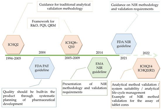
Figure 1. Guidelines used for the quality management of pharmaceutical products.
PAT is an indispensable unit in the newly emerging continuous manufacturing technologies and is required to demonstrate the process state of control and detect quality variations. Continuously recorded data enables the detection of process deviations and supports the root cause analysis of such events and the opportunity for continuous improvement [8].
Drug products present a complex quality profile built around multiple critical quality attributes (CQAs) influenced by controlled (formulation and process) and uncontrolled factors. A multivariate approach to product/process understanding is critical due to the complex interactions between these input factors affecting product quality. Moreover, these factors are likely to have different influence patterns between several quality attributes. To efficiently describe and understand these influences, a Design of Experiments-based development with response surface methodology is recommended [3,4].
If the recorded data accounts for multiple factors influencing that particular response, predicting complex quality attributes from PAT data can be managed appropriately from only one data source. Under these circumstances, the variation of any influential factor will be captured/perceived in the process analytical data and contribute to the method’s robust predictive performance. Thus, to obtain a robust monitoring performance, it is essential to identify the PAT tool sensible to these factors or to fuse multiple process analytical data.
The readily available advanced analytical platforms provide large amounts of diverse data associated with manufacturing processes that can be used for monitoring and predictive purposes. The challenge, in this case, refers to the integration of data from different sources to maximize the advantages of complementary information. The underlying idea/notion in performing data fusion (DF) is that the result of the fused dataset will be more informative than the individual datasets. Thus, this procedure will provide a more enhanced overview of the studied system with a more in-depth understanding and data-driven decision-making [9,10,11].
Implementing the DF concept in PAT represents the next step in the evolution of process monitoring technology that could provide a more comprehensive understanding of the system and the opportunity to predict complex quality attributes of drug products. Probably, due to the more strictly regulated field of the pharmaceutical industry, the use of this concept in drug manufacturing has been limited to some extent.
2. Data Fusion
2.1. Classification and Comparison of Fusion Methods
Several aspects exist that are used to classify the fusion methods/strategies in the terminology. Joint Directors of Laboratories (JDL) Data Fusion Group worked out a model that deals with the categorization of the information and DF. Castanedo systematized the classification of the DF techniques and strategies [69]. The divisions can be created by several criteria; however, the widespread classification used to accept in analytical chemistry follows the abstraction level of the input data [70]. The three levels are named after the complexity of the processing of the inputs from the data sources. Thus, low-, medium- and high-level DFs are distinguished (Figure 2).
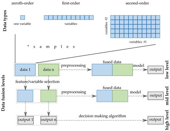
Figure 2. -DF strategies and data structures.
Low-level data fusion (LLDF) is considered the simplest method to achieve a combination of inputs. In this case, the data is rearranged into a new data matrix, where the variables coming from different sources are placed one after the other. The columns, i.e., the variables of the combined data matrix, will be the sum of the previously separated data sets. Usually, the concatenated data are then pretreated before creating the final classification or regression models. However, specific elementary operations can be conducted before putting them together [17].
Medium-(mid-)level data fusion (MLDF) (also called “feature-level” fusion) is based on a preliminary feature extraction that continues to maintain the relevant variables, eliminating the not sufficiently diverse, non-informative variables from the datasets. There are many developed algorithms to select these features or make the data reduction before merging them into one matrix that will be used in a chemometric method [71].
The high-level data fusion (HLDF) (also called “decision-level” fusion) works on a decision level. This means that the first step is to fit some supervised models to each data matrix. These models consist of regression models providing continuous responses for the input data or classifications, deciding the class membership of the new samples. The decisions from these models are combined into a complex model that can create the final estimation. The main idea behind HLDF is that the optimal regressions and classifications are built up for the different data types. Accordingly, a better estimation may be reached by unifying the outputs in one decision model.
Selecting and implementing an appropriate fusion method can prove to be a laborious task and should be driven by the considered application and the structure of the input data. To provide an effective comparison of the method’s performance in different setups (application type/input data structure), a literature survey was performed using studies that compare different fusion levels. Considering the pharmaceutical industry, the main areas of application of DF would include classification, regression, and process control, whereas regarding the data structure, mainly zero- and first-order data are encountered. Thus, all these factors/criteria were considered in the survey.
LLDF predominated as a suitable DF option under process control applications, where primarily multiple zero-order datasets were fused for multivariate- (MSPC) or batch statistical process control (BSPC) purposes (Figure 3). This strategy also proved effective for regression applications to merge several first-order datasets. Therefore, the fusion of data with a similar structure was efficient without applying a feature extraction procedure, as the similar structure avoided the predominance of one dataset over the other. Increased performance of LLDF was also attributed to the existence of complementary information between the datasets, which was maintained during the fusion procedure (not lost during feature extraction) [72]. Having more complementary information will be beneficial for reducing uncertainty.
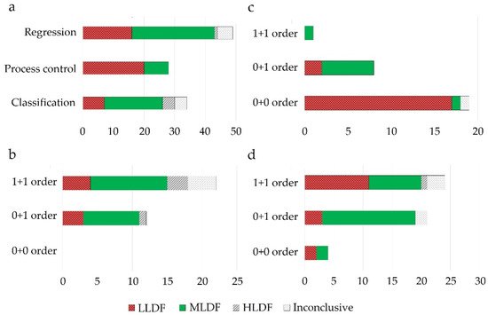
Figure 3. Evaluation of the best performing DF strategies across different areas of application (a) and their selection according to the data structure used for modeling ((b)-classification, (c)-process control, (d)-regression applications); 0 + 0: fusion of zeroth order data; 0 + 1: fusion of zeroth order data with first order data; 1 + 1: fusion of first-order data; x-axis represents the number of studies.
In some situations, instrument complementarity (not data complementarity) was not sufficient to improve the performance of predictive several CQAs, as shown by a Raman and FT-IR data based food analytical study [73].
As LLDF involves the concatenation of individual blocks at the level of original matrices after proper preprocessing, the dataset will contain many variables, some with increased predictive power, and also large parts of irrelevant data [72]. The ratio of predictive and uninformative variables obtained by adding new data can be disadvantageous as the noise can cancel out the advantages of valuable information [11,74,75]. Thus, the model building can become time-consuming and requires high computational power, although this limitation was overcome by using extreme learning machine modeling with a fast learning speed [76].
Assis et al. found the LLDF superior to MLDF when fusing NIR with total reflection X-ray fluorescence spectrometry (TXRF) data, highlighting the importance of scaling and variable selection procedure on the fused dataset. Autoscaling outperformed the block-scaling approach, and a variable reduction procedure was essential to eliminate redundant information [77]. A similar method was found appropriate by Assis et al. when ATR-FTIR and paper-spray mass spectrometry (PS-MS) data were combined [78].
Li et al. also demonstrated the superiority of LLDF over MLDF when NIR and MIR data were fused. The partial loss of relevant information during feature extraction affected MLDF performance [79]. As both LLDF and HLDF approaches relied on using the full spectral range, the developed models were superior to MLDF [79]. In this respect, the disadvantage of MLDF refers to the requirement of thoroughly investigating various feature extraction methods by developing multiple individual models [72,74]. However, the time invested in this stage is compensated by the more efficient model development using the extracted features [80].
MLDF was preferred when first-order data was combined with a zero-order or another first-order dataset (Figure 3). MLDF outperformed other fusion strategies when the feature extraction methods successfully excluded the uncorrelated variables.
If the extraction of features does not lead to the loss of predictive information, the MLDF strategy can offer a more accurate model and improved stability [81]. Therefore, the desired outcome of feature extraction is to maximize the amount of predictive variable content and minimize data size [82].
MLDF can offer a more balanced representation of variability captured in each dataset, especially when the number of variables is considerably large. The increased stability and robustness of MLDF over LLDF were also described in other studies [75,83,84]. The high level of redundant information found in LLDF data, negatively affected the synergistic effect of the fusion for different datasets [75,82,85].
A huge amount of information is involved when handling spectroscopic data. Thus, feature extraction is frequently implemented. Perfect classification of sample origin was achieved by separately extracting features from three different spectroscopic analysis techniques (NIR, fluorescence spectroscopy, and laser-induced breakdown spectroscopy (LIBS)) [86]. A similar discrimination model with successful identification was demonstrated for tablets using LIBS and IR spectra and MDLF [87].
Among the three areas of application, HLDF was selected as the best performing mainly in the case of classification applications when fusing first-order datasets (Figure 2). The utility of HLDF was also highlighted under similar input conditions in the case of regression applications (Figure 3).
Li et al. demonstrated that the synergistic effect of fusing data (FT-MIR; NIR) was achieved only when the valuable part of the data was used. LLDF was poorly performing due to the increased content of useless data, whereas the best classification strategy relied on HLDF [82]. The application dependency for selecting the fusion strategy has been recognized in other studies [72]. Another NIR and MIR-based application demonstrated the superior performance of HLDF, as the LLDF led to the loss of complementary information in the large dataset. At the same time, the MLDF approach gave mixed results depending on the evaluated response [11]. The use of the entire dataset over extracted features was the reason for HLDF superiority in another study [79].
In a previous study, LLDF caused no progression in classification, as presumably the analytical methods and sensors had dissimilar efficiency and provided noisy and redundant data [88]. Therefore, each output of the models had to be considered with different weights to make the final decision.
The advantages of HLDF are linked to its user-friendliness [11], and the possibility to easily update models with new data sources increases the versatility [89].
2.2. Data Processing
Regardless of the specific goal of the DF, the data measured by the analytical tools and sensors must be processed by various methods before building up chemometric models.
Firstly, the data sets might have different sizes, scales, and magnitudes. This can be handled by normalization and standardization to rescale the values into a range or to zero mean and unit variance. Autoscaling could be an appropriate solution for the fusion of univariate sensors with multivariate data, which frequently occurs in chemical or pharmaceutical processes [90,91,92,93]. The min-max normalization is suitable for MS [94] and some vibrational spectroscopic data [86,95]. It is typical to use normalization methods or elemental peak ratios for LIBS data to minimize the variability of replicates [96].
In the absence of differences in the measurement scale, additional preprocessing methods (scaling methods) will not be necessary, as the chance of dominating behavior will be reduced. This situation was encountered when mid-wave infrared (MWIR) and low-wave infrared (LWIR) data recorded by the same device were fused [72].
Secondly, the data, especially the spectral data, is usually influenced by the external interferences and measuring conditions causing different backgrounds, noise, and offset. Many well-known methods exist to increase the robustness of the datasets and, later, the models. Savitzky–Golay smoothing (SGS) is a commonly used method for noise reduction in spectra [79,85,97]. Several methods are proposed to tackle additive and/or multiplicative effects in spectral data. Background correction (BC) [98], Multiplicative Scatter Correction (MSC) [99], and Standard Normal Variate (SNV) [82,100] Unit area and vector normalization [98] are possible transformation methods to compensate for these effects. First or second derivatives are beneficial for enhancing the slight changes, thus, separating peaks of overlapping bands [40,75,101].
Thirdly, a dimensionality reduction step is essential to extract relevant features in MLDF [91,102,103]. Another justification for this step is to reduce the computational time during model development, i.e., for neural networks [104,105].
The applied feature extraction strategies identified in the literature survey can be divided into feature selection procedures relying on algorithms for selecting a sub-interval of the original dataset or on dimensionality reduction procedures, such as projection methods [76]. Moreover, their combined use has been demonstrated to have positive results in some situations [75,78,85]. The feature extraction methods applied in the literature survey for first-order data are presented in Figure 4.
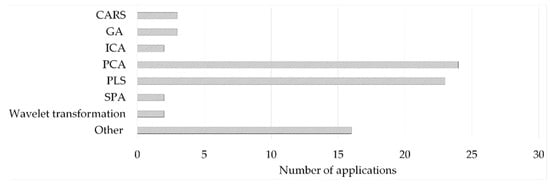
Figure 4. (Other—1 entry/method: 2D-image based estimator; correlation-based feature selection-CFS; forward selection; IRIV; multivariate curve resolution-alternating least squares (MCR-ALS); PARAFAC; Random frog (RF); Spectral signatures and leaf venation feature extraction; spectral window selection (SWS); T2, Q—derived from NIR-based MSPC; UV; variable selection based on the normalized differences between reference and sample spectral data; Variables Combination Population Analysis and Iterative Retained Information Variable Algorithm—VCPA-IRIV).
The measured data, particularly the spectral data, often include irrelevant variables that should be separated from the initial variables. Variable selection algorithms eliminate noisy spectral regions and redundant information to increase predictive accuracy [75]. In this respect, several methods derived from partial least squares (PLS) have been used. The synergy interval PLS (SI-PLS) algorithm was applied to select optimal subintervals and exclude unwanted sources of variation before a feature extraction step [75,85]. De Oliviera et al. reduced the variable numbers from LIBS and NIR spectra below 1% by recursive PLS (rPLS) and used them for DF purposes [106].
Uninformative and noise affected variables have been excluded using interval-PLS (i-PLS) [107,108]. As i-PLS continuously selects the variables, it should not be applied when the original data are not continuous (i.e., MS spectra) [78]. The use of variable importance in the projection (VIP) and i-PLS has also been reported [100].
The VIP-based variable ranking has shown efficacy in filtering unimportant variables and reducing variable space [84,108,109]. Generally, a VIP > 1 is considered relevant, although this limit has no statistical meaning [84,99,110]. In this respect, Rivera-Perez et al. identified discriminant variables through VIP and an additional statistical significance criterium (p < 0.05) from ANOVA or t-tests [111].
The use of genetic algorithm (GA), iteratively retained informative variables (IRIV), competitive adaptive reweighted sampling (CARS), successive projections algorithm (SPA), recursive feature extraction (RFE), univariate filter (UF), and ordered predictors selection (OPS) has also been reported [78,86,94,108,110,112,113]. GAs have been used in spectroscopic applications for optimal wavelength selection, multicollinearity, and noise reduction [108]. The algorithm selects an initial set of spectral variables, which is further optimized by testing multiple combinations of different features. The comparison between GA and UF [113], respectively, and GA and OPS variable selection methods has been investigated for DF applications [78].
The fine-tuning of variables can be dealt with individually for each data set at the statistical significance level, through Pearson correlation analysis [114]. Another option that enables the extraction of features from spectroscopic data is wavelet transformation. During this procedure, the original signal is decomposed considering different wavelet scales, resulting in a series of coefficients [115]. Wavelet compression was used for the fusion of spectral data from different sources [107], while other studies fused different scale-based wavelet coefficients generated from the same input data [115].
The other big category of feature extraction methods relies on estimating a new set of variables. Projection methods were the most frequently applied feature extraction tools to reduce the dimensionality and remove unwanted correlation. More than 60% of the studies included in this survey used either Principal component analysis (PCA) or PLS for this purpose during the development of fusion-based models. Both techniques are based on the coordinate transformation of the original n × λ sized dataset (where n is the number of observations and λ is the number of variables) by combining the original variables. In the case of PCA, this is performed in the way that the new variables (i.e., principal components, PCs) are orthogonal, and the first few variables describe the possible highest variance in the dataset. For PLS, the new variables (latent variables, LVs) maximize the covariance with the dependent variables. For more details, the reader is referred to, e.g., [116] and [117]. Other feature extraction methods found in the literature are parallel factor analysis (PARAFAC), a generalization of PCA [91], independent component analysis (ICA) [118], orthogonal-PLS [104], or autoencoder [119].
The obtained LVs have been extensively used as relevant features for DF applications [118,120,121,122]; for overview purposes [104] and outlier identification [72].
The use of latent variables as extracted features has to consider the size of captured variability [96,104,105]. In this respect, several significance criteria have been used for selecting relevant PCs, including the percentage of explained original data (R2X) [82,123], the eigenvalue [104] or the predictive performance during cross-validation (RMSECV) [124,125]. Some applications excluded the possibility of discarding relevant PCs and fused multiple latent variables, independent of their significance [76,126,127]. However, such an approach increases the risk of overfitting.
The use of the Gerchberg–Saxton algorithm has also been reported to establish the optimal number of feature components [75].
Several studies found PLS to be a superior feature extraction method, as it was possible to emphasize the spectral variability correlated with the response of interest [125,128]. For example, Lan et al. extracted the features of interest from NIR spectra by developing PLS models having as a response the components of interest determined by HPLC [110].
The separation of spectral variability into predictive and orthogonal parts can be achieved using orthogonal-PLS (OPLS). As a result, the feature extraction can efficiently exclude uncorrelated variations from the input data [104]. Although it would appear beneficial to use only the predictive components, non-predictive parts can have a positive effect on performance results due to the intra-class correlations from different sources [129].
PLS-DA (PLS-Discriminant analysis), another extension of PLS, has also been applied for feature extraction [74], by either generating latent variables [11] or by selecting a small set of representative variables [80].
2.3. Modeling Methods
PCA and PLS regression can be regarded as the most widespread chemometric tools [130]; consequently, the literature survey highlighted the predominance of projection methods in the modeling of fused datasets (Figure 5). PLS-DA and PCA were the preferred modeling choice for classification applications, followed by the support vector machine (SVM), soft independent modeling using class analogy (SIMCA), linear discriminant analysis (LDA), k-nearest neighbors (kNN), or artificial neural networks (ANN) (Figure 5a). For process control applications, PLS models were mainly used to develop batch evolution/level models having process maturity (time-variable) or a CQA of the product as response variables (Figure 5b). PLS was also the preferred modeling option for regression applications, followed by ANN and SVM methods (Figure 5c).
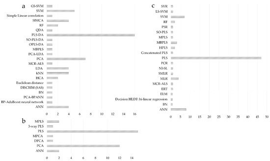
Figure 5. Evaluation of modeling methods considered for classification (a); process control (b) and regression purposes (c); x-axis represents the number of studies using a particular method.
In the case of LLDF, PCA and PLS modeling can be directly applied to analyze the different data sources. This is an especially suitable method when univariate sensor data are fused, such as in [131], as the computational demand of the model might increase significantly when several multivariate data (e.g., spectra with thousands of variables) are handled together. Nevertheless, it is also possible to concatenate different spectra for developing a single PCA or PLS model. For example, mid- and long-wave NIR spectra could be incorporated into the same PLS model to utilize the information of the whole IR range [72]. The only difference between PCA/PLS models developed for DF—compared to a single-source model—is that additional preprocessing steps might be necessary to compensate for the possible scale differences.
Several extensions of the traditional PCA/PLS concept account for the structured nature of the fused dataset. For instance, Multiblock-PLS (MB-PLS) provides block scores, as well as relative importance measures for the individual data blocks instead of accounting for the whole concatenated data [132]. Although the prediction itself does not improve compared to the traditional PLS model, it significantly contributes to the interpretability of the model. For example, the block weights and scores have helped identify the most critical variables in an API fermentation [133]. In other studies, MB-PLS and the “block importance in prediction (BIP)” index were used to determine which PAT sensors (IR, Raman, laser-induced fluorescence-LIF spectroscopy, FBRM, and red green blue-RGB color imaging), process parameters, and raw material attributes are necessary to be included in the DF models [134,135]. Malechaux et al. demonstrated that a multiblock modeling approach was superior to hierarchical PLS-DA, as the simple concatenation of NIR and MIR data presented a small fraction of predictive variables compared to the complete dataset [11]. Other multiblock modeling methodologies are also promising, such as the response-oriented sequential alternation (ROSA), which facilitates handling many blocks [136]. It was also possible to include interactions in the model [137]. However, to the best of the authors’ knowledge, these approaches have not been utilized for real-life PAT problems.
For MLDF, it was demonstrated that both feature extraction and modeling steps significantly impact the model performance and, therefore, need to be optimized carefully [11,104]. For PAT data, a typical combination of methods is the application of individual PCA models for feature extraction and using the concatenated PC scores in a PLS regression model [72]. Besides PC scores, process/material parameters can also be conveniently incorporated into the PLS model, improving the model compared to the LLDF of the analytical sensor data [103]. Similarly, MSPC models can also be employed [10,103].
Another approach is the utilization of sequential methods in which the order of data blocks will be important for modeling. Most feature extraction procedures use an independent approach, meaning that each data source is processed individually, and the blocks are exchangeable. Foschi et al. used Sequential and Orthogonalized-Partial Least Squares-Discriminant Analysis (SO-PLS-DA) algorithm to classify samples through NIR and MIR data [138]. The algorithm builds a PLS model from the first data block and aims to improve the model’s performance using orthogonal (unique) information from the next data block. This sequential approach removes redundant information between datasets and extracts information to give an optimal model complexity [138].
After the features are derived from the raw data, ANNs can also serve as the DF model, which performed superior to PLS regression in multiple studies [104,105,139]. It was also possible to develop a cascade neural network using PCA scores to predict the quantitative process variables (i.e., component concentrations) of fermentation and then to evaluate the process state, e.g., determine the harvest time [140]. Compared to PLS, ANN and SVM have the advantage of being more suitable in the presence of non-linearity [85,104,141].
HLDF deduces a unique outcome from the results of multiple models, which are built with individual data sources. Consequently, the method requires decision support systems, which incorporate numerous versatile methods, e.g., sensitivity, uncertainty, and risk analysis [142]. Moreover, in the QbD concept, the design space is defined as the multi-dimensional combination and interaction of critical material and process parameters that are demonstrated to assure quality. That is, it could be regarded as an HLDF model when the critical input parameters are monitored with individual PAT tools and chemometric models. Design spaces could be defined by several methods, such as response surface fitting, linear and non-linear regression, first-principles modeling, or machine learning [143,144,145].
Independently of the fusion level, deep learning is another emerging modeling method for PAT data but has been neglected [62]. The structure of the deep neural networks enables the fusing of raw data (low-level), extracting features (mid-level), and making decisions (high-level) adaptively in a single model [146]. Several deep learning solutions can be found in the literature for DF in different industrial processes but not yet for pharmaceutical processes. For example, convolutional neural networks (CNN) could be used for fault diagnosis [147,148] or soft sensing in the production of polypropylene [149]. It has also been demonstrated that support vector machines, logistic regression, and CNNs could be used to fuse laser-induced breakdown spectroscopy (LIBS), visible/NIR hyperspectral imaging, and mid-IR spectroscopy data at different levels [119]. Therefore, their applications in pharmaceutical tasks could be further studied in the future.
This entry is adapted from the peer-reviewed paper 10.3390/molecules27154846
This entry is offline, you can click here to edit this entry!