Artificial Intelligence in Glaucoma

Artificial Intelligence in Glaucoma: History

View Latest Version

Please note this is an old version of this entry, which may differ significantly from the current revision.

Subjects: Ophthalmology

Contributor: Antonio Maria Fea , Federico Ricardi ,

Cristina Novarese

, Francesca Cimorosi ,

Veronica Vallino

, Giacomo Boscia

Glaucoma is a multifactorial neurodegenerative illness requiring early diagnosis and strict monitoring of the disease progression. Artificial intelligence algorithms can extract various optic disc features and automatically detect glaucoma from fundus photographs.

biomarkers
artificial intelligence
genetics

1. Artificial Intelligence in Glaucoma

The use of artificial intelligence is expanding rapidly. Machine learning (ML) and deep learning (DL) allowed a more sophisticated and self-programming way to use machines in automatic data analysis. More in detail, in machine learning, a system can automatically improve its performance and learn by itself with experience without being specifically programmed to do so. Specifically, using a convolutional neural network (CNN) architecture, the deep learning algorithm can take in an input image, assign importance (learnable weights and biases) to various aspects/objects in the image, and be able to differentiate one from the other [5]. Similar to neurons derived from the mammalian visual cortex, the neural network’s architecture consists of many hidden layers, each with its specific receptive field and connection to a further layer (Figure 1).

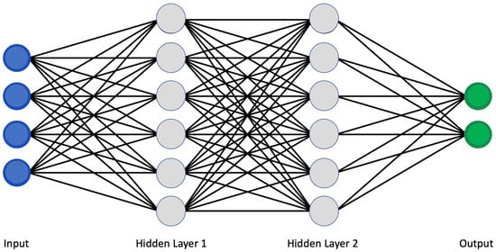
Figure 1. Classical scheme of a convolutional neural network.

The deep learning network works as a two-step process. The first is the feature learning step, in which convolution, pooling, and activation functions make the ‘jump ahead’ between hidden layers. Secondly, the classification function converts the probability value to a label, providing a clinical output such as healthy or pathologic [6,7].

Although this architecture traditionally provided a high degree of computational power, in recent years, more advanced network architectures have been developed, allowing the system to analyze more complex data sources. AlexNet (2012) was introduced to improve the results of the ImageNet challenge. VGGNet (2014) was introduced to reduce the number of parameters in the CNN layers and improve the training time. ResNet (2015) architecture makes use of shortcut connections to solve the vanishing gradient problem (which is encountered when during the iteration of training, each of the neural network’s weights receives an update proportional to the partial derivative of the error function with respect to the current weight) [8]. The basic building block of ResNet is a residual block that is repeated throughout the network. There are multiple versions of ResNet architectures, each with a different number of layers. Inception (2014) increases the network space from which the best network is to be chosen via training. Each inception module can capture salient features at different levels [9].

Traditional metrics assessing the DL algorithm’s quality are sensitivity, specificity, precision, accuracy, positive predictive value, negative predictive value, and area under the receiver operating curve (AUC).

It is known that the early detection of glaucoma could eventually preserve vision in affected people. However, due to its clinical history of being symptomatic only in advanced stages and when most of the RGCs are already compromised, it is crucial to introduce a tool to detect glaucoma in clinical practice in pre-symptomatic form automatically. Furthermore, it could be of clinical relevance also to find new ways to provide targeted treatment and forecast the clinical progression.

2. Fundus Photography

In clinical practice, ophthalmologists suspect glaucoma by analyzing optic nerve head (ONH) anatomy, cup-to-disc ratio (CDR), optic nerve head notching or vertical elongation, retinal nerve fiber layer (RNFL) thinning, presence of disc hemorrhages, nasal shifting of vessels, or the presence of parapapillary atrophy. However, the diagnostic process could be challenging considering the extreme variance of these parameters [10]. It has been shown that agreement among experts on detecting glaucoma from optic nerve anatomy is barely moderate [11]. Furthermore, with standard fundus photography, not only the variability of anatomy could be misleading, but also the parameters of acquisition such as exposition, focus, depth of focus, contrast, quality, magnification, and state of mydriasis.

In this scenario, artificial intelligence algorithms can extract various optic disc features and automatically detect glaucoma from fundus photographs. For example, Ting et al. [7] collected 197,085 images and trained an artificial intelligence algorithm to automatically determine the cup-disc ratio (CDR) with an AUC of the receiver operating characteristic (ROC) curve of 0.942 and sensibility and specificity, respectively, of 0.964 and 0.872. Similarly, Li et al. [12] developed an algorithm based on 48,116 fundus images reporting high sensitivity (95.6%), specificity (92.0%), and AUC (0.986). Although the importance of automatically detecting the excavation of the optic nerve head, it is known that high inter-subject variability characterizes CDR; some large optic nerve heads have bigger cupping even without any sign of glaucoma. To reduce the rate of false positives, other researchers trained a deep learning algorithm to determine the presence of glaucoma based on fundus photographs and implemented it with the visual field severity [13].

Li and coworkers used a pre-trained CNN called ResNet101 and implemented it with raw clinical data in the last connected layer of the network; interestingly, there were no statistically significant changes in AUC, but they found an improvement in the overall sensitivity and specificity of the model, confirming the importance of multi-source data to improve the discriminative capacity of the glaucomatous optic disc [14].

More recently, Hemelings et al. utilized a pre-trained CNN structure relying on active and transfer learning to develop an algorithm with an AUC of 0.995. They also introduced the possibility for clinicians to use heatmaps and occlusion tests to understand better the predominant areas from which the algorithm based its predictions; it is an exciting way of trying to overcome some problems related to the well-known ‘black-box’ effect [15].

The majority of the publications that were analyzed suggested that an automated system for diagnosing glaucoma could be developed (Table 1). The severity of the disease and its high incidence rates support the studies that have been conducted. Deep learning and other recent computational methods have proven to be promising fundus imaging technologies. Some recent technologies, such as data augmentation and transfer learning, have been used as an alternative way to optimize and reduce network training, even though such techniques necessitate a large database and high computational costs.

Table 1. Summary of studies on glaucoma detection using fundus photography.

Author	Year	N. of Images	Structure	SEN	SPEC	ACC	AUC
Kolar et al. [16]	2008	30	FD			93.80%
Nayak et al. [17]	2009	61	Morphological	100%	80%	90%
Bock et al. [18]	2010	575	Glaucoma Risk Index	73%	85%	80%
Acharya et al. [19]	2011	60	SVM			91%
Dua et al. [20]	2012	60	DWT			93.3%
Mookiah et al. [21]	2012	60	DWT, HOS	86.7%	93.3%	93.3%
Noronha et al. [22]	2014	272	Higher order cumulant features	100%	92%	92.6%
Acharya et al. [23]	2015	510	Gabor transform	89.7%	96.2%	93.1%
Isaac et al. [24]	2015	67	Cropped input image after segmentation	100%	90%	94.1%
Raja et al. [25]	2015	158	Hybrid PSO	97.5%	98.3%	98.2%
Singh et al. [26]	2016	63	Wavelet feature extraction	100%	90.9%	94.7%
Acharya et al. [27]	2017	702	kNN (K = 2) Glaucoma Risk index	96.2%	93.7%	95.7%
Maheshwari et al. [28]	2017	488	Variational mode decomposition	93.6%	95.9%	94.7%
Raghavendra et al. [29]	2017	1000	RT, MCT, GIST	97.80%	95.8%	97%
Ting et al. [7]	2017	494,661	VGGNet	96.4%	87.2%		0.942
Kausu et al. [30]	2018	86	Wavelet feature extraction, Morphological	98%	97.1%	97.7%
Koh et al. [31]	2018	2220	Pyramid histogram of visual words and Fisher vector	96.73%	96.9%	96.7%
Soltani et al. [32]	2018	104	Randomized Hough transform	97.8%	94.8%	96.1%
Li et al. [12]	2018	48,116	Inception-v3	95.6%	92%	92%	0.986
Fu et al. [33]	2018	8109	Disc-aware ensemble network (DENet)	85%	84%	84%	0.918
Raghavendra et al. [29]	2018	1426	Eighteen-layer CNN	98%	98.30%	98%
Christopher et al. [34]	2018	14,822	VGG6, Inception-v3, ResNet50	84–92%	83–93%		0.91–0.97
Chai et al. [35]	2018	2000	MB-NN	92.33%	90.9%	91.5%
Ahn et al. [36]	2018	1542	Inception-v3 Custom 3-layer CNN			84.5% 87.9%	0.93 0.94
Shibata et al. [37]	2018	3132	ResNet-18				0.965
Mohamed et al. [38]	2019	166	Simple Linear Iterative Clustering (SLIC)	97.6%	92.3%	98.6%
Bajwa et al. [39]	2019	780	R-CNN	71.2%			0.874
Liu et al. [40]	2019	241,032	ResNet (local validation)	96.2%	97.7%		0.996
Al-Aswad et al. [41]	2019	110	ResNet-50	83.7%	88.2%		0.926
Asaoka et al. [42]	2019	3132	ResNet-34				0.965
			ResNet-34 without augmentation				0.905
			VGGI I				0.955
			VGGI 6				0.964
			Inception-v3				0.957
Kim et al. [43]	2019	1903	Inception-V4	92%	98%	93%	0.99
Orlando et al. [44]	2019	1200	Refuge Data Set	85%	97.6%		0.982
Phene et al. [45]	2019	86,618	Inception-v3	80%	90.2%		0.945
Rogers et al. [46]	2019	94	ResNet-50	80.9%	86.2%	83.7%	0.871
Thompson et al. [47]	2019	9282	ResNet-34				0.945
Hemelings et al. [15]	2020	8433	ResNet-50	99%	93%		0.996
Zhao et al. [48]	2020	421	MFPPNet				0.90
Li et al. [49]	2020	26,585	ResNet101	96%	93%	94.1%	0.992

ARCH = Architecture; SEN = Sensibility; SPEC = Specificity; ACC = Accuracy; AUC = Area under the curve.

3. Optical Coherence Tomography

Optical coherence tomography (OCT) is an essential tool to capture not only the glaucomatous optic disc in two dimensions (2D) but to provide a three-dimensional (3D) visualization, including the deeper structures. It is a technique based on the optical backscattering of biological structures; it has been widely adopted to assess glaucoma damage both on the anterior segment (e.g., with anterior segment OCT to detect angle closure) and posterior segment (e.g., with traditional OCT to detect ONH morphology and RFNL thickness) [50].

For this reason, depending on the input data, it is possible to differentiate five subgroups of deep learning models: (1) models for prediction of OCT measurements from fundus photography, (2) models based on traditionally segmented OCT acquisitions, (3) models for glaucoma classification based on segmentation-free B-scans, (4) models for glaucoma classification based on segmentation-free 3D volumetric data and (5) models based on anterior segment OCT acquisitions.

Thompson et al. showed that it is possible to predict the Bruch membrane opening-based minimum rim width (BMO-MRW) using optic disc photographs with high accuracy (AUC was 0.945) [51]. Similarly, other researchers reported a high AUC for their model to predict RNFL thickness from fundus images [52,53,54]. Asaoka et al. developed a CNN algorithm to diagnose glaucoma based on thickness segmentations of RNFL and ganglion cells with inner plexiform layer (GCIPL) [42,55]. Wang et al. used 746,400 segmentation-free B-scans from 2669 glaucomatous eyes to automatically develop a model to detect glaucoma with an AUC of 0.979 [56].

Maetschke et al. [57] developed a DL model with an AUC of 0.94 using raw unsegmented 3D volumetric optic disc scans. Similarly, Ran et al. [58] validated a 3D DL model based on 6921 OCT optic disc volumetric scans; the AUC was 0.969, with a comparable performance between the model and glaucoma experts. Russakoff et al. used OCT macular cube scans to train a model to classify referable from non-referable glaucoma; despite the quality of the model, it did not perform as expected on external datasets [59].

At last, DL models based on AS-OCT have been developed to detect the presence of primary angle closure glaucoma (PACG), such as the one proposed by Fu et al. [60]. Xu et al. further developed this type of algorithm to predict the PACG as well as the spectrum of primary angle-closure diseases (PACD) (e.g., primary angle-closure suspect, primary angle-closure) [61].

The papers cited clearly demonstrated that using DL on OCT for glaucoma assessment is effective, precise, and encouraging (Table 2). Despite that, prior to implementing DL on OCT monitoring, more research is required to address some current challenges, including annotation standardization, the AI “black box” explanation problem, and the cost-effective analysis after integrating DL in a real clinical scenario.

Table 2. Summary of studies on glaucoma detection using OCT technology.

	Author	Year	Outcome Measures	Arch	SEN	SPEC	ACC	AUC
OCT Fundus	Thompson et al. [47]	2019	1. Global BMO-MRW prediction	ResNet34				0.945
			2. Yes glaucoma vs. No glaucoma
	Medeiros et al. [53]	2019	1. RNFL thickness prediction	ResNet34	80%	83.7%		0.944
			2. Glaucoma vs. Suspect/healthy
	Jammal et al. [52]	2020	RNFL prediction	ResNet34				0.801
	Lee et al. [62]	2021	RFNL prediction	M2M
	Medeiros et al. [54]	2021	Detection of RFNL thinning from fundus photos	CNN
OCT 2D	Asaoka et al. [55]	2019	Early POAG vs. no POAG	Novel CNN	80%	83.3%		0.937
	Muhammad et al. [63]	2017	Early glaucoma vs. health/suspected eyes	CNN + transfer learning			93.1%	0.97
	Lee et al. [64]	2020	GON vs. No GON	CNN (NASNet)	94.7%	100%		0.990
	Devalla et al. [65]	2018	Glaucoma vs. normal	Digital stain of RNFL	92%	99%	94%
	Wang et al. [56]	2020	Glaucoma vs. no glaucoma	CNN + transfer learning				0.979
	Thompson et al. [51]	2020	POAG vs. no glaucoma	ResNet34	95%	81%		0.96
			Pre-perimetric vs. no glaucoma		95%	70%		0.92
			Glaucoma with any VF loss (perimetric) vs. no glaucoma		95%	80%		0.97
			Mild VF loss vs. no glaucoma		95%	85%		0.92
			Moderate VF loss vs. no glaucoma		95%	93%		0.99
			Severe VF loss vs. no glaucoma		95%	98%		0.99
	Mariottoni et al. [66]	2020	Global RNFL thickness value	ResNet34
OCT 3D	Ran et al. [58]	2019	Yes GON vs. No GON	CNN (NASNet)	89%	96%	91%	0.969
					78–90%	86%	86%	0.893
	Maetschke et al. [57]	2019	POAG vs. no POAG	Feature-agnostic CNN				0.94
								0.92
	Russakoff et al. [59]	2020	Referable glaucoma vs. non-referable glaucoma	gNet3D-CNN				0.88
AS-OCT	Fu et al. [60]	2019	Open angle vs. Angle closure	VGG-16 + transfer learning	90%	92%		0.96
	Fu et al. [67]	2019	Open angle vs. Angle closure	CNN				0.9619
	Xu et al. [61]	2019	1. Open angle vs. angle closure	CNN (ResNet18) + transfer learning				0.928
			2. Yes/PACD vs. no PACD					0.964
	Hao et al. [68]	2019	Open angle vs. Narrowed Angle vs. Angle closure	MSRCNN				0.914

ARCH = Architecture; SEN = Sensibility; SPEC = Specificity; ACC = Accuracy; AUC = Area under the curve.

SEN = Sensibility, SPEC = Specificity, ACC = Accuracy, AUC = Area under the curve.

4. Standard Automatic Perimetry

Visual field testing represents a fundamental exam for diagnosing and monitoring glaucoma. In distinction from the fundus photographs and OCT, it allows the interpretation of the functionality of the whole visual pathway. Given the importance of visual function testing for the detection and clinical forecast of glaucoma, many researchers recently developed DL algorithms using the complex quantitative data it contains. Asaoka et al. [69] trained a DL algorithm to automatically detect glaucomatous visual field loss with an AUC of 0.926; the performance of their model was higher if compared to other machine learning classifiers methods, such as random forests (AUC 0.790) and support vector machines (AUC 0.712).

Elze et al. [70] employed archetypal analysis technology to obtain a quantitative measurement of the impact of the archetypes or prototypical patterns constituting visual field alterations. Similarly, Wang et al. developed an artificial intelligence approach to detect visual field progression based on spatial pattern analysis [71].

Given the importance of predicting visual loss patterns in glaucoma patients, specifically for prescribing a personalized treatment, researchers have developed interesting tools to predict the probability of disease progression based on visual field data. DeRoos et al. [72] were able to compare forecasted changes in mean deviation (MD) on perimetry at different target pressures using a machine-learning technique called Kalman Filtering (KF). KF is a machine-learning technique derived from the aero-spatial industry that compares the course of the disease of a single patient to a population of patients with the same chronic disease; in this scenario, it could potentially predict the rate of conversion to glaucoma in patients with ocular hypertension as well as disease progression in the future for patients with manifest glaucoma (Table 3). [73,74].

Table 3. Summary of studies on artificial intelligence applied to visual field testing.

Author	Year	Outcomes Mesures	Architecture	SEN	SPEC	ACC	AUC
Asaoka et al. [69]	2016	Pre-perimetric VFs vs. VFs in healthy eyes	FNN				0.926
Kucur et al. [75]	2018	Early glaucomatous VF loss vs. no glaucoma	CNN with Voronoi representation
Li et al. [12]	2018	Glaucomatous VF loss vs. no glaucoma	VGG I 5	93%	83%	88%	0.966
Li et al. [76]	2018	Glaucoma vs. Healthy	VGG	93%	3%		0.966
Berchuck et al. [77]	2019	Rates of VF progression compared to SAP MD; Prediction of future VF compared to point-wise regression predictions	Deep variational autoencoder
Wen et al. [78]	2019	HFA points and Mean Deviation	CascadeNet-5
Kazemian et al. [74]	2018	Forecasting visual field progression	Kalman Filtering Forecasting
Garcia et al. [73]	2019	Forecasting visual field progression	Kalman Filtering Forecasting
DeRoos et al. [72]	2021	Forecasting visual field progression	Kalman Filtering Forecasting

The possibility of low-cost screening tests for the disease has been made possible by the consistent demonstration of deep learning models’ ability to detect and quantify glaucomatous damage using standard automated perimetry automatic assessment. Additionally, it has been demonstrated that DL enhances the evaluation of the damage on unprocessed visual field data, which could enhance the utility of these tests in clinical practice. As already stated, the validation of new diagnostic tests, despite how exciting AI technologies may be, should be based on a rigorous methodology, with special attention to the way the reference standards are classified and the clinical settings in which the tests will be adopted.

This entry is adapted from the peer-reviewed paper 10.3390/ijms24032814

© Text is available under the terms and conditions of the Creative Commons Attribution (CC BY) license; additional terms may apply. By using this site, you agree to the Terms and Conditions and Privacy Policy.