Precision agriculture or precision farming is the targeted application of crop input according to the locally determined crop needs. Therefore, it is the geo-referenced application of crop inputs, whose rates must be strictly those required by the crop. The most essential points of information about the topic being described are: overview; brief history of precision agriculture; theoretical basics of precision agriculture; precision agriculture cycle; geo-referenced measurement of within-field parameters; analysis and interpretation of geo-referenced data for mapping within-field parameters; spatially variable rate application of crop inputs; instruments for precision agriculture; current scenario of precision agriculture; current scenario of precision viticulture; Global Navigation Satellite Systems (GNSS) and differential correction technique; proximal sensors of within-field soil and crop parameters; remote sensing from Unmanned Aerial Vehicles (UAVs) and satellites; devices for setting up and controlling spatially variable rate crop input application; assisted guidance systems of agricultural machines; perspectives of precision agriculture.
- environmental protection
- within-field crop and soil parameters
- within-field spatial variability
- crop inputs
- GNSS
- proximal sensors
- remote sensing
- GIS
- setting up and control devices
- guidance systems of agricultural machines
1. Introduction
The within-field spatial variability is the variation of the soil and/or crop parameters of a field, from a point to another of the field itself.
The within-field soil parameters are the following:
- structure;
- cone penetrometer resistance (or tenacity);
- depth of the layer to be cultivated;
- texture;
- pH;
- nutrients contents;
- water content;
- organic matter content;
- microflora (bacteria) and microfauna;
- weeds;
- parasites (fungi, bacteria and insects) and pathologies.
The within-field crop parameters are the following:
- plant biomass;
- vegetative vigour;
- yield;
- production quality.
Any field shows a significant spatial variability of at least one of its parameters.
Traditional agriculture is based on the application of a spatially uniform rate of each crop input, without taking into account the within-field spatial variability. Therefore, traditional agriculture causes high environmental impact and production cost.
Precision agriculture takes into account the within-field spatial variability and, therefore, is based on the application of spatially variable rates of each crop input. Therefore, precision agriculture is environmentally friendly.
The benefits of precision agriculture are the following:
- environmental (reduction of environmental impact, due to lower used amounts of crop inputs);
- energetic (reduction of consumed fuels and oil and, indirectly, reduction of used amounts of chemical fertilisers);
- economical (improvement of quality and quantity production and, above, reduction of the used amounts of crop inputs, that, together with the decreased used amounts of fuels and oil, results in the reduction of production cost) [1].
2. History of Precision Agriculture
In order to reduce the environmental impact and optimise the use of crop inputs, precision agriculture was born.
Precision agriculture was born after that the USA Department of Defense (DoD) made available Global Positioning System (GPS) not only to military users but also to civilian ones, in 1983.
In fact, precision agriculture (technology for producing yield maps) was implemented for the first time in US, in the Corn Belt of Mid West, to herbaceous crop rotations, at the beginning of 1980s.
Precision agriculture was implemented for the first time in Europe, in England, to herbaceous crop rotations, at the end of 1980s: John P. Fenton used a combine harvester Massey Ferguson MF 38, mounting a gamma-ray yield sensor, in his farm of North Yorkshire, in 1988 (Figure 1).
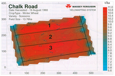
Figure 1. Yield map of “Chalk Road” field (1993), divided into three management zones, where different fertiliser rates were applied.
The technology for producing yield maps was implemented to cereal crops in Australia at the beginning of 1990s.
The first combine harvesters mounting yield mapping technology was commercialised in Europe in 1997.
Precision agriculture was firstly implemented in Italy at the end of 1990s, i.e. to a crop rotation corn-soybean-corn-common wheat-soybean, in the farm “San Basilio” of Ariano Polesine (Rovigo), in 1998.
Precision agriculture was implemented to herbaceous crops by means of:
- yield mapping technology, including yield sensors (of cereals, i.e. wheat and corn, sugar beet and potato) and humidity sensors;
- spatially variable rate (nitrogen - N, phosphorous - P, potassium - K) fertiliser application.
The grapevine yield maps were produced in California (US), in the counties of Sonoma Russian Valley and Sonoma Coast AVAs, in the farm of Paul and Kathiryn McGrath Sloan, in 1998.
The first grape yield sensors were commercialised in 1999.
Rob Bramley produced yield maps of the territories of Clare Valley, Coonawarra, Padthaway, and Riverlands regions of South Australia district and Sunraysia region of Victoria district (Australia), in 1999 and 2000.
Meanwhile the Selective Availability (SA), that is a positioning error (distance between the position of a point on the earth surface measured by a positioning system and its actual position) of 100 m (in 95% of measurements) introduced in GPS by USA Department of Defense (DoD), was removed on the 1st of May 2000.
The spatially variable vineyard management was implemented in Italy, in the farms of Cantine (cellars) Giacomo Montresor of Cavalcaselle (Verona) and Riccagioia of Torrazza Coste (Pavia), in 2001 and 2002, respectively.
Precision agriculture was implemented to grapevine by means of:
- vegetative vigour mapping technology (e.g. remote sensing from satellites);
- yield mapping technology (e.g. grape yield, sugar content and total acidity sensors);
- spatially variable crop operations (e.g. green pruning and harvest).
The geo-referenced sensing of vineyard parameters is aimed at discovering its areas having a different NDVI (Normalised Difference Vegetation Index), index of vegetative vigour, and/or a different product quality (e.g. grape sugar content and total acidity). It is possible to perform a spatially variable green pruning or harvest, depending on the grape ripening level.
Pellenc and Gregoire manufacturers started to commercialise machines able to implement precision viticulture, i.e. machines for wood pruning and grape harvesters (Figure 2) [1].
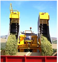
Figure 2. Grape harvester equipped with two hoppers for spatially variable harvest in two areas having different vegetative vigour.
3. Theoretical Basics of Precision Agriculture
The theoretical basics of precision agriculture are described in the following subsections.
3.1. Precision Agriculture Cycle
The precision agriculture cycle (Figure 3) comprises the following three phases:
- geo-referenced measurement of within-field parameters;
- analysis and interpretation of geo-referenced data for mapping within-field parameters;
- spatially variable rate application of crop inputs [1].
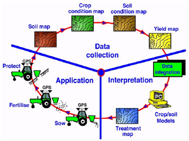
Figure 3. Precision agriculture cycle [1].
3.1.1. Geo-Referenced Measurement of Within-Field Parameters
The geo-referenced measurement of within-field crop and soil parameters can be implemented by means of proximal sensors or remote sensing.
Proximal sensors can be distinguished according to their working principle, while remote sensing can be performed by using images taken by Unmanned Aerial Vehicles (UAVs) or satellites.
3.1.2. Analysis and Interpretation of Geo-Referenced Data for Mapping Within-Field Parameters
The analysis and interpretation of the several geo-referenced data of each crop and soil within-field parameter (big data) is the most difficult challenge of precision agriculture.
This phase is aimed at producing maps of within-field crop and soil parameters and, then, spatially variable rate crop input application maps, by means of a GIS (Geographic Information System) software.
3.1.3. Spatially Variable Rate Application of Crop Inputs
The application of all crop inputs can be:
- spatially uniform rate;
- localised (aimed at rows);
- spatially variable rate.
The spatially variable rate application of crop inputs is the final phase of precision agriculture cycle.
3.2. Instruments for Precision Agriculture
The following instruments are needed for implementing precision agriculture:
- GNSS (Global Navigation Satellite Systems), for sensing the position to which any measured within-field parameter must be tagged (phase 1) and that where the rate of a crop input must be applied (phase 3);
- sensors, for measuring the within-field crop and soil parameters (phase 1);
- GIS software, for producing the maps of within-field crop and soil parameters, as well as those for the application of spatially variable rates of crop inputs, and other software for interpreting the measured data (phase 2);
- models of soil-crop simulation, for identifying the causes of within-field spatial variability (phase 2);
- devices, for setting up and controlling the application of spatially variable rates of crop inputs (phase 3) [1].
3.3. Current Scenario of Precision Agriculture
Precision agriculture is spread only in large areas of Northern America (USA) and Northern Europe (Germany, Denmark, Netherlands and United Kingdom).
In Northern America and United Kingdom “on-the-go” sensors of within-field crop parameters (e. g. GreenSeeker in USA, Yara N-Sensor in United Kingdom) and remote sensing are used for spatially variable rate nitrogen fertiliser application in herbaceous crops.
In Northern America “on-the-go” sensors of within-field crop parameters (e.g. WeedSeeker in USA) are used for spatially variable rate herbicide application in herbaceous crops.
In Italy precision agriculture is implemented in only 1% of Utilised Agricultural Area (UAA) [2].
Precision agriculture is, above all, applied to herbaceous crops by means of: technology for producing crop yield maps; spatially variable rate fertiliser and herbicide application [1].
3.4. Current Scenario of Precision Viticulture
Precision agriculture is applied also to tree crops and, above all, to grapevine, by means of:
- technology for producing vegetative vigour maps, allowing to plan spatially variable pruning;
- technology for producing crop yield maps, allowing to plan temporary variable harvest, in the vineyard management zones having different ripening periods, or spatially variable harvest, in the management zones having different levels of vegetative vigour;
- spatially variable crop operations (e.g. green pruning, fertilisation, fungicide treatments and harvest) [1].
3.5. Global Navigation Satellite Systems (GNSS) and Differential Correction Technique
The following satellite constellations (Figure 4) are currently available for precision agriculture:
- GPS (USA), 31 satellites;
- GLONASS (Russia), 22 satellites;
- EGNOS (UE), SBAS (Satellite-Based Augmentation System) developed by European Space Agency (ESA) within Galileo project, 25 satellites;
- BeiDou (China), 48 satellites;
- QZSS or MSAS (Japan), 4 satellites;
- IRNSS (India), 7 satellites.
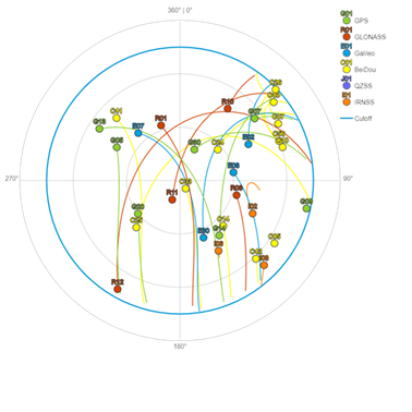
Figure 4. Sky plot (https://www.gnssplanning.com) (Trimble).
In order to minimise the positioning error, i.e. the distance between the position of a point on the earth surface measured by a GNSS and its actual position, it is needed to implement a differential correction technique.
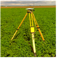
A differential correction technique needs two GNSS receivers (Figure 5), instead of one:
- base station, to be used as single one or belonging to a network of RTK base stations (EUREF Permanent Network - EPN in Europe), comprising e.g. a GPS/GLONASS dual frequency (L1 - 1575,42 MHz / L2 - 1227,60 MHz but also L2C / L5 - 1176,45 MHz) receiver, having e.g. 220 channels (for receiving 220 satellite signals), and a radio transmitter having a frequency of 450 or 900 MHz, for transmitting differential correction data, and a powering battery (e.g. having a maximum autonomy of 10 hours);
- mobile receiver or rover, e.g. a GPS/GLONASS dual frequency (L1 / L2 but also L2C / L5) one, having e.g. 220 channels, and a radio receiver, having a frequency of 450 or 900 MHz, for receiving the differential correction data from a base station.
A

B
Figure 5. GNSS receivers to be used for differential correction technique: (a) base station; (b) mobile receiver (Trimble).
3.6. Proximal Sensors of Within-Field Soil and Crop Parameters
The on-the-go or real time proximal sensors of within-field soil and crop parameters can be distinguished into five categories, according to their working principle, as shown in Table 1 [3].
Table 1. On-the-go proximal sensors 1 of within-field soil and crop parameters [3].
|
Soil and crop parameters |
Electrical or electro-magnetical |
Optical or radiometrical |
Mechanical |
Acustic or pneumatic |
Electro-chemical |
|
compaction or bulk density |
|
|
X (c) |
X |
|
|
mechanical resistance |
|
|
X (c) |
|
|
|
shear strength |
|
|
X |
|
|
|
draft force |
|
|
X (c) |
|
|
|
depth of soil or soil pan |
X |
|
X |
X |
|
|
texture |
X (c) |
X (c) |
|
X |
|
|
pH |
|
X |
|
|
X (d, c) |
|
salinity or sodium (Na) content |
X (c) |
|
|
|
X |
|
water volume content |
X (c) |
X (c) |
|
|
|
|
organic matter or carbonium (C) content |
X |
X (c) |
|
|
|
|
residual nitrate or nitrogen (N) content |
X (c) |
X |
|
|
X (d) |
|
other macronutrients (e.g. soluble potassium - K - content) |
|
|
|
|
X (d) |
|
Cationic Exchange Capacity (CEC) |
X |
X (c) |
|
|
|
|
weed distribution |
|
X (c) |
X |
|
|
|
plant biomass |
|
X (c) |
X |
|
|
|
vegetative vigour |
|
X |
|
|
|
|
deficiency level of nutrients |
|
X (c) |
|
|
|
|
yield of cereals and other crops (e.g. soybean, rapeseed, sugarbeet, potato and grapevine) |
X |
X |
X (d) |
|
|
|
production quality (e.g. grain proteins) |
|
X |
|
|
|
1 d = sensors for direct measurement (all the others are sensors for indirect measurement); c = commercial sensors (all the others are experimental sensors).
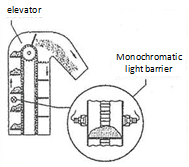
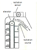
In order to measure the yield of cereals, a yield sensor must be mounted on the combine harvester, at the top of the elevator (auger) of the clean grain (Figure 6) [4].
A
B
Figure 6. Two yield sensors for combine harvesters: (a) optical yield sensor that, combined with a humidity sensor, can achieve an error of 3% ca. and is affected by the field slope; (b) yield sensor equipped with gamma ray detector that, combined with a humidity sensor, can achieve an error of 1% ca. [4].
3.7. Remote Sensing from Unmanned Aerial Vehicles (UAVs) and/or Satellites
In order to remotely sense the vegetative vigour of crop plants, it is needed to obtain the images taken in the phenological phases when a variation of the value of a vegetative index (e.g. Normalised Difference Vegetation Index - NDVI, that is an index of vegetative vigour) is supposed, as shown in Table 2.
Table 2. Phenological phases of some tree and herbaceous crops for remote sensing.
|
Crop |
January |
February |
March |
April |
May |
June |
July |
August |
September |
October |
November |
December |
|
Grapevine |
|
|
|
Before green pruning |
After green pruning |
|
|
Before harvest |
After harvest |
|
|
|
|
Olive |
Before pruning |
After pruning |
|
Before flowering |
After flowering |
|
|
|
|
|
Before harvest |
After harvest |
|
Almond |
|
|
Before vegetative awakening |
After vegetative awakening |
|
|
Before harvest |
After harvest |
|
|
|
|
|
Durum wheat |
|
Before raising |
After raising |
|
Before harvest |
After harvest |
|
|
|
Aftre seeding |
|
|
|
Oregano |
|
|
|
After transplanting |
|
Before harvest |
After harvest |
|
|
|
|
|
|
Stevia rebaudiana |
|
|
|
After transplanting |
|
Before harvest |
After harvest |
|
|
|
|
|
It is needed to select the vegetative indexes to be remotely sensed (e.g. NDVI) and, when the weather factors (e.g. wind) are favourable, let the UAV (Figure 7) fly on the cultivated fields. Thus, it is possible to remotely sense images and, after processing, produce maps of each vegetative index for each field.
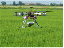
Figure 7. Unmanned Aerial Vehicle (UAV) equipped with a multispectral camera and a GNSS mobile receiver (ARVAtec).
As far as a possible protocol for remote sensing from UAVs, for each species the sampling of plant leaves should be carried out, by randomly collecting the leaves of four levels of vegetative activity, in a specific area (e.g. 1 ha ca.): 1) maximum; 2) intermediate higher; 3) intermediate lower; 4) minimum.
The sampling points can be identified by means of row numbers and plant numbers (e.g. grapevine, cultivar Syrah, fruit tree form step-over espalier, plant distances 2.5 x 1 m).
The result of the chemical analysis of each collected sample is the nitrogen content of the considered species for the considered level of vegetative activity.
After taking the images, a map of the vegetation index can be produced.
For each species and for any value from -1 to +1, at intervals of 0.25, the sampling of leaves should be carried out, in order to determine the nitrogen content for any value of the vegetation index and, therefore, validate the remotely sensed data.
The same value of nitrogen content can be associated with any point of the map characterised by the above value of the vegetation index.
The map of the vegetation index can be converted in a map of nitrogen content and, then, based on the nitrogen demand by that species, in a nitrogen application map and, finally, based on the nitrogen content of the fertiliser to be used, in a theoretical spatially variable rate nitrogen fertiliser application map.
Yet, when the field area is higher than 5 ha, the images acquired by satellites can be cheaper than those taken by UAVs.
Moreover, the use of a UAV, equipped with a multispectral camera and a GNSS (e.g. GPS, GLONASS and EGNOS) mobile receiver, implies an initial investment, as well as having qualified staff able to set up and pilot this device and performing subsequent processing of the obtained data, while satellite imagery providers offer ready-to-work images, as well as the possibility of consulting the images archive.
The satellite Copernicus Sentinel-2 (Figure 8) takes images with a spatial resolution of 10 m and a temporal resolution of five days, so that it provides maps of NDVI and NDWI (Normalised Difference Water Index, i.e. index of leaf water content) every five days.
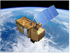
Figure 8. Satellite Copernicus Sentinel-2.
In fact, it is possible to convert the images remotely sensed by the satellite Copernicus Sentinel-2 (e.g. provided by the Portoguese web-based platform AgroInsider) into maps of within-field crop and soil parameters and, then, spatially variable rate crop input application maps.
Thus, remote sensing from UAVs and/or satellites is useful as Decision Support System (DSS) for both precision and traditional agriculture, e.g. for deciding if, when and how spatially variable rate fertiliser and/or water application must be performed in a field.
In fact, remote sensing from satellites can be used for:
- deciding if spatially variable rate fertiliser management must be performed in a field, based on the eventual within-field spatial variability of plant vegetative vigour;
- deciding if spatially variable rate irrigation must be performed in a field, based on the eventual within-field spatial variability of plant leaf water content (only for remote sensing from satellites);
- identifying the optimal fertilisation and irrigation time (only for remote sensing from satellites), based on the comparison between the graph of plant vegetative vigour and that of plant leaf water content (also for spatially uniform rate fertilisation and irrigation, within traditional agriculture);
- determining the spatially variable fertiliser rate to be applied in each management zone, based on the within-field spatial variability of plant vegetative vigour;
- determining the spatially variable water rate to be applied in each management zone, based on the within-field spatial variability of plant leaf water content (only for remote sensing from satellites);
- identifying two or three areas of different levels of vegetative vigour inside each plot, e.g. high, medium and low, so that the grapes harvested in these areas can be processed for producing different wines having different quality.
However, the two above image sources, i.e. UAVs and satellites, can be combined as DSSs, in order to contribute to spatially variable crop management, according to the principles of precision agriculture [5].
3.8. Devices for setting up and controlling spatially variable rate crop input application
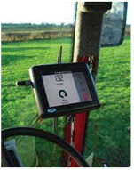
A controller of the electronic setting up system having distribution proportional to the forward speed (Figure 9) can be mounted on a centrifugal or pneumatic fertiliser spreader or a sprayer, in order to:
- apply fertiliser or pesticide mixture rates by relying on a theoretical spatially variable rate application map, that was previously produced and logged in the on-board computer (setting up);
- log the applied rates of the crop input, in order to produce the actual spatially variable rate application map (control).
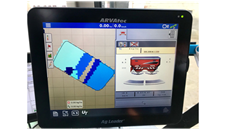
Figure 9. InCommand 1200 controller of the electronic setting up system having distribution proportional to the forward speed of Ag Leader (ARVAtec).
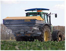
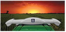
In order to perform the on-the-go spatially variable rate fertiliser application, it is needed to use the Yara N-Sensor (Figure 10), mounted on the roof of tractor cab. It can measure the light reflectance by the leaves of the cultivated plants and, indirectly, their chlorophyll content. The difference between the nitrogen needed for the crop and the indirectly measured nitrogen content will be the amount of nitrogen to be applied, and, by relying on the nitrogen content of the fertiliser, its rate. The on-board computer transmits the corresponding input to the setting up and control system of the fertiliser spreader.
The Yara N-Sensor ALS 2 (Active Light Source) (Figure 11a) is an active sensor having its own multispectral light source (flashing Xenium lamp). This system allows to perform spatially variable rate nitrogen fertiliser application also under conditions of poor or no (by night) light intensity.
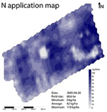
If one of the two above devices for setting up and controlling spatially variable rate crop input application comprises also a GNSS receiver, it is possible to produce an actual spatially variable rate fertiliser application map (Figure 11b).
A
B
Figure 10. System for on-the-go spatially variable rate fertiliser application: (a) Yara N-Sensor mounted on the cabin roof of a tractor connected to a centrifugal fertiliser spreader; (b) on-board computer inside the tractor cab (Yara).
A
B
Figure 11. System for on-the-go spatially variable rate fertiliser application: (a) Yara N-Sensor ALS 2 (Yara); (b) actual spatially variable rate fertiliser application map.
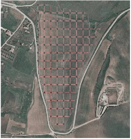
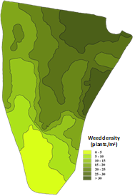
In order to perform the spatially variable rate herbicide application, a field base map must be firstly produced by means of a GNSS receiver and a GIS, in order that a grid can be overlapped on this map (Figure 12a). Thus, any grid vertex identifies the centre of a circle area of weed sensing. Through interpolation (linear, of nearest point, Kriging) of the amount of weed plants per area unit it is possible to produce a weed density map.
The weed density map (produced through linear interpolation) shows areas having different density of these plants (Figure 12b).
A
B
Figure 12. Procedure for spatially variable rate herbicide application: (a) overlap of a grid on a field base map for identifying the circular areas where weeds were monitored; (b) weed density map [6].
By tagging to each weed density a specific rate of herbicide mixture to be applied it is possible to produce the theoretical spatially variable rate herbicide map (Figure 13a).
The electronic setting up system having distribution proportional to forward speed allows to log the applied rates of herbicide mixture and tag them to positions, in order to produce an actual spatially variable rate herbicide application map (Figure 13b) [6].
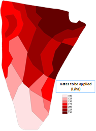
A
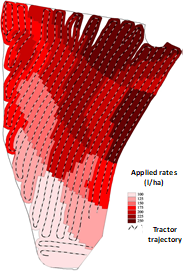
B
Figure 12. Procedure for spatially variable rate herbicide application: (a) theoretical spatially variable rate herbicide application map; (b) actual spatially variable rate herbicide application map [6].
In order to perform the on-the-go spatially variable rate herbicide application, it is needed to use the WeedSeeker (Trimble) (Figure 13), that can be mounted on the front part of a tractor connected to a sprayer. It measures the presence of weed plants and sends the corresponding input to each nozzle, in order that this applies a determined rate of herbicide mixture only on weeds, before seeding or after harvest. This system works at a speed up to 16 km/h and uses optical sensors able to sense the presence of weeds.
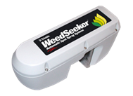
Figure 13. The WeedSeeker can be mounted on the front part of a tractor connected to a sprayer for performing a on-the-go spatially variable rate herbicide application (Trimble).
3.9. Assisted Guidance Systems of Agricultural Machines
The modern guidance systems of agricultural machines can be distinguished in two categories:
- semi-automatic or free hands guidance systems;
- automatic or autopilot guidance systems.
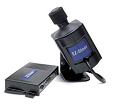
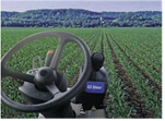
In a semi-automatic or free hands guidance system, the driver moves the steering wheel during the advance along a road, while an electrical pilot can move the steering wheel during a crop operation (Figure 14). This system allows the driver to pay attention to the working quality of the agricultural implement and increase the forward speed by 10-15% (e.g. soil tillage by means of rotary tiller and seeding).
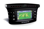
A
B
C
Figure 14. Semi-automatic guidance system: (a) EZ-Guide computer; (b) controller and Ez-Steer electrical pilot; (c) Ez-Steer electrical pilot, mounted on the steering wheel (Trimble).
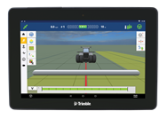
Recently automatic guidance systems (unmanned systems) allow to accutately follow planned trajectories along a field, in order to perform offsets of the machine position and correct its steering angle (Figure 15). During a crop operation, a controller moves the steering wheel, the gearbox, the hydraulic lift and the agricultural machine or implement connected to the tractor.

A

B
C

D
 E
E
Figure 15. Automatic guidance system: (a) GNSS NAV-900 mobile receiver; (b) Autosense optical steering angle sensor; (c) Trimble GFX-750 computer; (d) Navigation Controller II; (e) T3 electronic valve (Trimble).
The benefits of the assisted guidance systems of agricultural machines are the following:
- application of crop inputs without overlapping or failure between consecutive passes (reduction of overlapping between consecutive passes by 5-10%);
- reduction of the amount of passes by 5-13% and, therefore, of the used amounts of crop inputs, as well as actual time;
- increase of the actual working width by 3-10%, as well as of the forward speed and, therefore, of the theoretical working capacity;
- more accurate soil tillage;
- reduction of soil compaction, through the passage of agricultural machines along planned trajectories (tramlines in Controlled Traffic Farming - CTF);
- reduction of fuel consumption and emission of Greenhouse Gases (GHGs, e.g. nitrous oxides);
- soil levelling (only by means of automatic guidance systems);
- improvement of safety, as some obstacles could cause even the tractor overturning and, therefore, the accident of the driver, above all under conditions of poor visibility;
- improvement of ergonomics, as the fatigue of the driver is reduced, as well as some obstacles can cause a reduction of driving comfort, besides an excessive wear and, therefore, an increase of extraordinary maintenance cost of the machine.
4. Perspectives of Precision Agriculture
Remote sensing (e.g. from Copernicus Sentinel-2 satellite) provides a high amount of information about soils and crops.
On the other hand the sensors of soil parameters can provide at low cost spatially dense data, that can be combined with the data produced by means of remote sensing, crop scouting, yield maps and Digital Elevation Models (DEMs), in order to: divide a field into management zones; drive soil sampling; improve the accuracy of spatially variable rate crop input application maps.
The results of most field tests of sensor-based nitrogen fertiliser management have often shown a 10-20% saving of the amount of this macronutrient.
For this crop operation, a future step will be the conversion of livestock manure (also together with other biowaste, e.g. household waste, wood sawdust, straw, hay, barley stalks, sunflower and/or wheat husks, walnut shells, wood chips, tree bark, cotton, tree stump, molasses, biochar and/or ash) into pellets, i.e. cylindrical granular fertilisers (by means of granulation plants or granulators), to be used for spatially variable rate biofertiliser application by means of centrifugal spreaders. Thus, it will be possible to solve, at the same time, the following problems, according to the principles of Circular Bioeconomy (CBE):
- high production of biowaste, e.g. livestock manure, that implies costs for storage, transport and application on soils, as well as bed smell and pathogens;
- replacement of expensive and highly energy consuming inorganic/mineral/chemical fertilisers with organic ones, not only able to increase the soil nutrient contents but also its organic matter content and, therefore, improve its structure and, finally, maximise the crop yield;
- increase of farmer profit, due to lower costs for manure management and fertiliser purchase;
- reduction of GHGs (e.g. biomethane) emission and bed smell, as well as removal of pathogens [7].
Moreover, sensors under development for weed detection vary from simple colour detectors to complex machine vision systems, aimed at using colour, shape and texture of plant materials, in order to both distinguish weeds from crops and identify different weed species.
Furthermore, soil-crop simulation models must be used for identifying the causes of within-field spatial variability and for decision-making, i.e. producing increasingly accurate spatially variable rate crop input application maps.
In the future precision agriculture could be implemented on a larger scale if the following requirements will be satisfied:
- to quantify its economic and environmental benefits;
- to develop user-friendly software for processing and interpreting the measured geo-referenced data (big data);
- to use electronic devices compatible among each other and an integrated user-friendly software for all spatially variable crop operations (commercialised by some manufacturers, yet);
- to develop soil-crop simulation models, in order to identify the causes of within-field spatial variability and, therefore, adjust the crop input rates from the next growing season [1].
References
- Comparetti, Antonio. Precision Agriculture: Past, Present and Future. In Proceedings of the International scientific conference Agricultural Engi-neering and Environment - 2011 “Agroinzinerija ir energetika Nr. 16 - 2011”, key-note presentation, Akademija, Kaunas district, Lithuania, 22-23 September 2011, ISSN 1392-8244; Aleksandras Stulginskis University: Kaunas, Lithuania, 2011; pp. 216-230.
- Blasi, Giuseppe; Pisante, Michele; Sartori, Luigi; Casa, Raffaele; Liberatori, Sandro; Loreto, Francesco; De Bernardinis, Bernardo; Furlan, Lorenzo; Guaitoli, Fabio; Sarno, Giampaolo. Linee Guida per lo Sviluppo dell’Agricoltura di Precisione in Italia (Guidelines for the Development of Precision Agriculture in Italy); Ministero delle Politiche Agricole, Alimentari e Forestali (Italian Ministry of Agricultural, Food and Forestry Policies): Rome, Italy, 2017; pp. 1-78.
- Adamchuk, Viacheslav I.; Hummel, John W.; Morgan, M.T.; Upadhyaya, Shrini K.; On-the-go sensors for precision agriculture. Computers and Electronics in Agriculture 2004, 44, 71-91, https://doi.org/10.1016/j.compag.2004.03.002.
- Carrara, Michele; Pessina, Domenico; Comparetti, Antonio; Orlando, Santo; Misurare la resa con precisione (Measuring the yield with precision). Terra e Vita 2004, 8, 63-66, .
- Comparetti, Antonio; Marques da Silva, Jose Rafael; Use of Sentinel-2 satellite for spatially variable rate fertiliser management in a Sicilian vineyard. Sustainability 2022, 14(3), 1-18, https://doi.org/10.3390/su14031688.
- Carrara, Michele, Comparetti, Antonio; Febo, Pierluigi; Orlando, Santo; Spatially variable rate herbicide application on durum wheat in Sicily. Biosystems Engineering 2004, 87(4), 387-392, https://doi.org/10.1016/j.biosystemseng.2004.01.004.
- Zinkevičienė, Raimonda; Jotautienė, Egle; Juostas, Antanas; Comparetti, Antonio; Vaiciukevičius, Edvardas; Simulation of granular organic fertilizer application by centrifugal spreader. Agronomy 2021, 11(2), 1-13, https://doi.org/10.3390/agronomy11020247.