Title of the project 

Lift force analysis to Glider MDM-1

This review article is part of the Emerging Tools Design project with Tomahawks aviation. The context of the subject is as follows: The subject takes place in a current collaboration between Tomahawks Aviation in Ergolding/Germany and the university of Wolverhampton. The goal is to improve the Fox MDM-1 glider so that it can drop loads via air drop. The problematic posed here in this report is to characterize the performances and characteristics of this aircraft with several results to expose.

In this report will be presented:

• The CAD of the aircraft
• CFD of the design glider
• CFD of the Seagull.SLDRT
• Interpretation and comparison of the results
• A decision matrix on the choice of materials used in the aircraft fuselage (at least 10 criteria)

Image Based CAD

The design of the following glider was made with SolidWorks 2022 a DASSAULT SYSTEME solution.

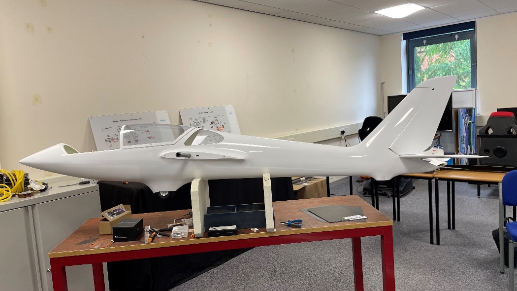
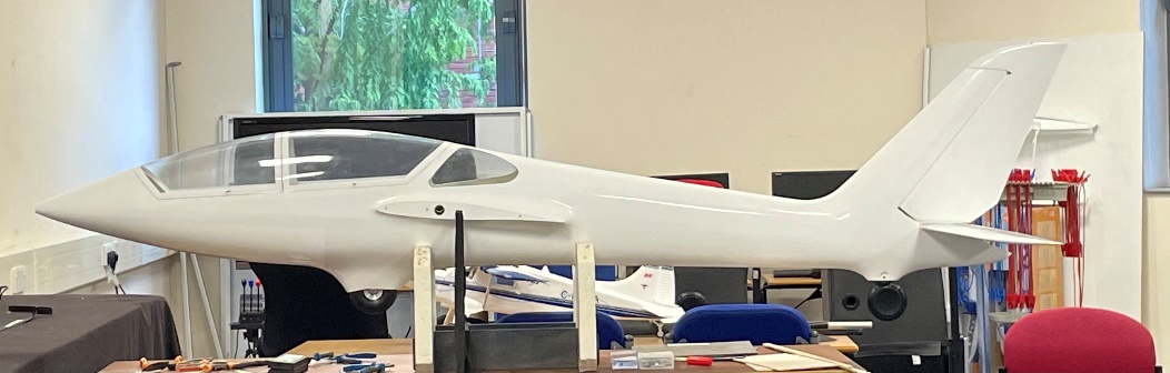
The first step was to take pictures of the aircraft. This one was disassembled, the fuselage on one side and the wing on the other. The enemy of image-based design is perspective. Indeed, the closer a picture is taken, the more the proportions around the center will be distorted. On the contrary, a photo taken from very far away will have a negligible perspective leaving the proportions homogeneous.

a)

b)

Figure 1 : Photo of the fuselage a) with important perspective, b) with reduce perpective and faithfull proportions

The photo a) is taken close to the glider while b) was taken at the other end of the room and then zoomed in. The proportions are more accurate on b) you can see it at the level of the cocpit but also the rear stabilizer.

All the pictures were taken with as much distance as possible but some of them are still too distorted like the wing for example (very large part)

Design

When designing an airplane, it seems logical to start the design with the fuselage, as one would start with the hull of a boat for example. So, the first step was to represent the main body of the fuselage without any artifice (no wheels, no interface with the wings and no stabilizers). The first difficulty was to calibrate the 2 pictures together. Once put together, the proportions are not the same, which forces to approximate some shapes and dimensions. Below the fuselage limits are drawn on 2 perpendicular planes and coincident at 2 points.

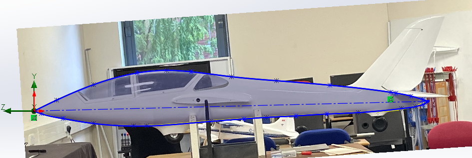
Figure : Right Plane sketch fuselage

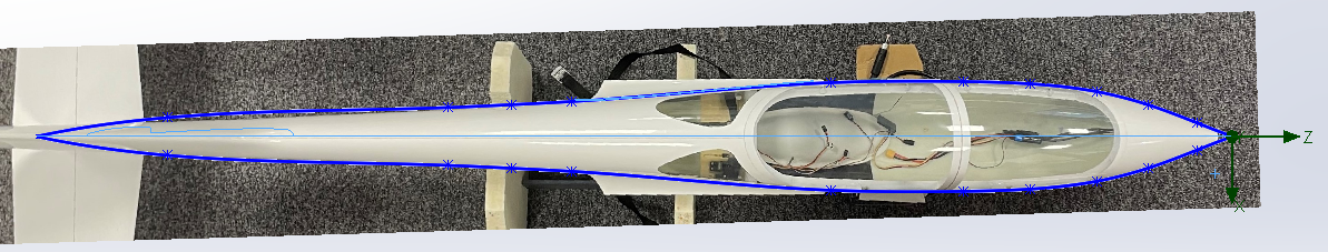
Figure : Top plane sketch fuselage

Then, the length was divided with 17 section planes. On each of them a sketch connects the 3 points (intersection between section plane and previous fuselage profiles) while keeping the tangency with the other half of the fuselage. The function used below builds almost the entire aircraft. It takes in input sections that will be projected between them following a closing point. And can also take for a better control, control curves that will govern the path of the projection between the sections.

Figure 4 : loft function for fuselage

Then, all the tailing is done with the LOFT function. The yellow and blue sections represent the profiles and the pink curves are the control curves.

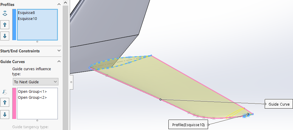
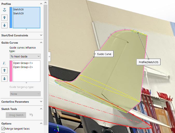
Figure : loft function for stabilisator

Figure 6 : loft function for tailplane

The design of the wing is the most important step of the design. Because we know that it is the wings that will generate the lift. It starts by designing the wing section. With a convex upper surface and a flat lower surface so that the air passing above has more path to travel than the air passing below. Another particularity, the leading edge has a larger diameter than the trailing edge which is Sharpe.

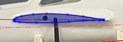
Figure 7 : Wing section

About the angle of attack of the wing, on the diagram above the red construction line represents the axis of the fuselage from nose to tail. The blue construction line represents the wing angle. You cannot change the angle between the wing and the fuselage, it is the photo that determines how the wing is placed in relation to the fuselage. However, for the simulation the angle between the blue construction line and the origin axis must be 6°. Here the angle between wing and fuselage is about 0.2° so before the simulation we will apply a rotation of 5.8° in X axis.

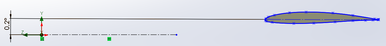
Figure 8 : Angle of attack between the wing and the fuselage (before simulation)

Then this section was extruded to model the interface between the fuselage and the wing.

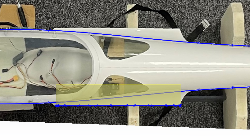
Figure 9 : Wing section extrusion for Fuselage/Wing interface

This part which precedes the wing has a particular shape and we will be able to reproduce it thanks to the function Variable Leave. We select the intersection between the extrusion and the fuselage because that is what we want to round off. Then we select 2 points (leading edge and trailing edge) where we will define different fillet radii, here 10 mm at the leading edge and 40 mm at the trailing edge.

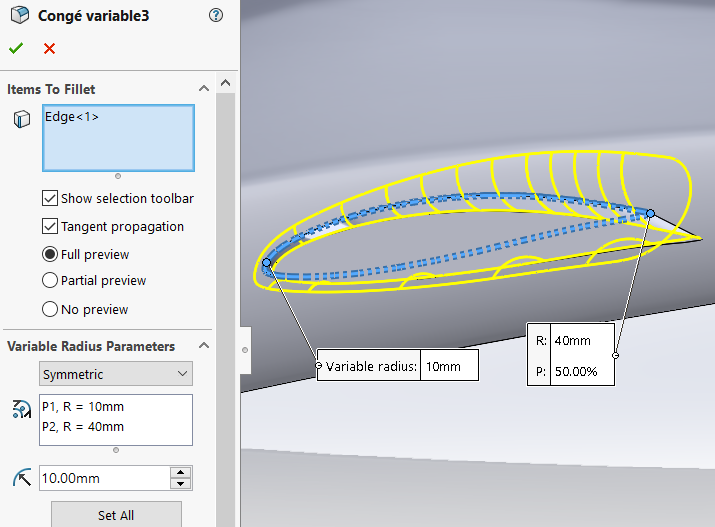
Figure 10 : Evolutive Fillet for the Wing/Fuselage interface

Now that the base is done, we can create the wing in the same way as a stabilizer, shifting a plane to the winglet level in which we will make a wing section smaller than the fuselage but still with the same shape. And we select the control curves that we have drawn thanks to the image of the wing. The choice of this background image is voluntary, my wing picture had too much perspective and it didn't match with the fuselage.

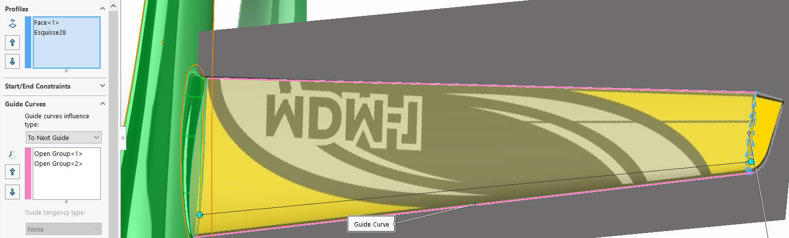
Figure 11 : Loft function for the Wing

On effectue la symétrie des éléments.

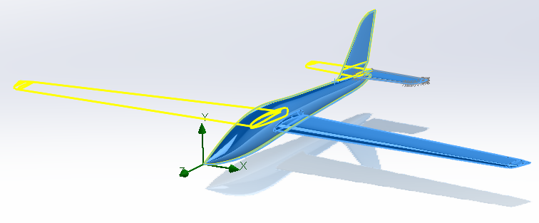
Figure 12 : Mirror function

Then we apply the 5.8° angle for all the plane so the angle of attack of the wing is surely 6°.

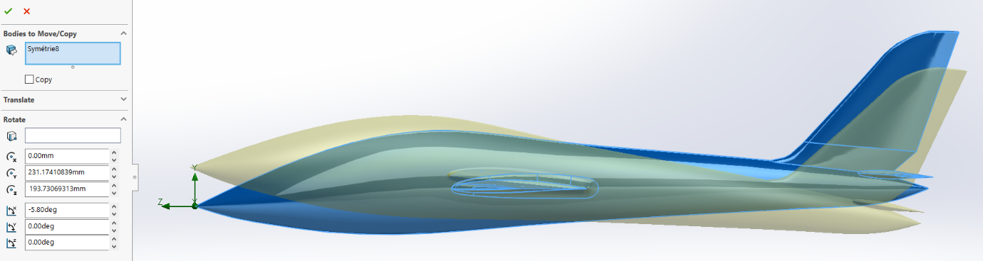
Figure 13 : Rotation function for all the glider

Here we evaluate the wingspan, it is good, 4.66m.

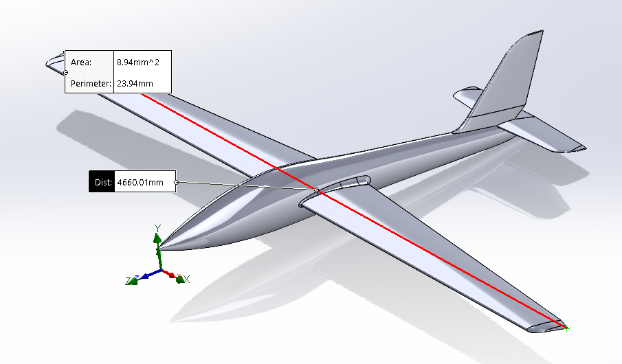
Figure 14 : Evaluation of the wingspan

Simulation

Simulation is a powerful tool that allows today's engineer to predict with a margin of error what will happen in any situation. Today it is impossible to simulate a system composed of thousands of moving parts and to extract all the data on a run. What engineers do is isolate the desired subsystem and apply boundary conditions that represent the links that this part has with the outside world (Fixation, bore, degree of freedom...) Therefore, if you don't apply the right boundary conditions, you misinterpret the physics around your subsystem, the simulation is worthless. It is a rigorous discipline. Below are the basic parameters of our simulation, surface roughness, air speed in the domain, pressure... this part is the same for the two following airplane.

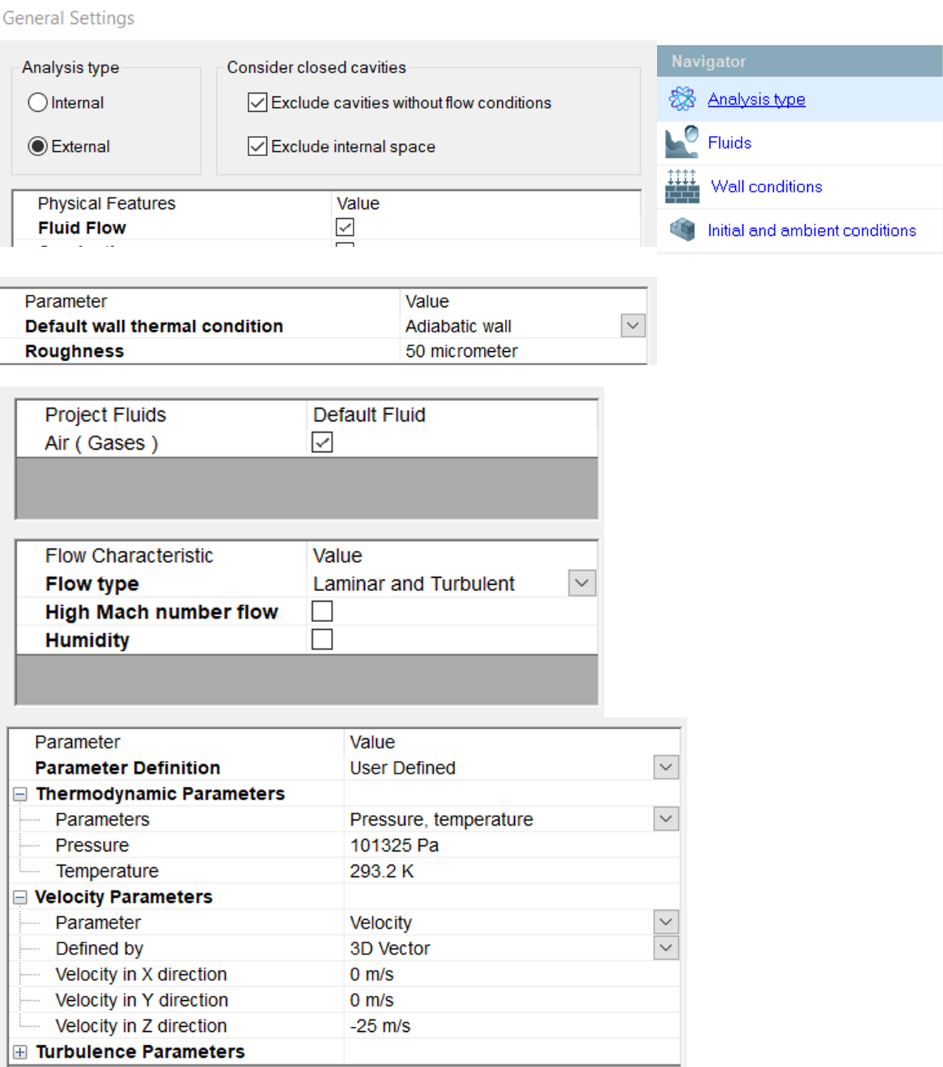
Figure 15 : Initial conditions for the simulation

Then we define a domain not too large (waste of computational resources) but not too small (so that all phenomena appear)

Figure 16 : Domain of the simulation study

Below we define a mesh, this is a very important step. Your mesh is a direct factor of the number of iterations generated and therefore of the calculation time and resources. It defines the precision of your results. Here the number of nodes allows us to make a calculation on the whole plane (1 part) in 5 minutes.

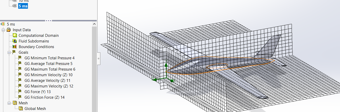
Figure 17 : Representation of the mesh

Then we launch the calculation, and we can observe in real time the iteration and the data as below

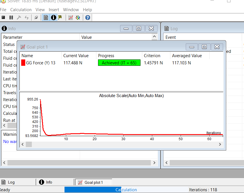
Figure 18 : Running calculation about Lift (value convergence)

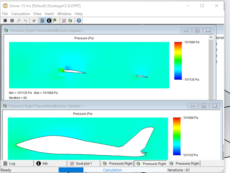
Figure 19 : Running calculation about the pressure field in two different plane

Results

Fox behaviour

In this part we will analyze and interpret the results obtained. These are presented in 3 forms, the cut plots, surface plot, and flow trajectory.

For the cut plots which will be presented to you are the cutting planes located at 0.4 meters from the origin in the direction of the wing see figure 20

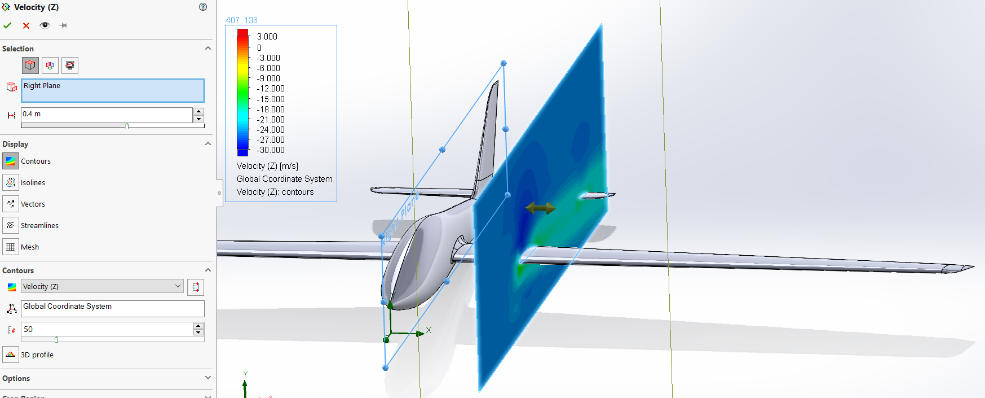
Figure 20 : Cut plot Definition

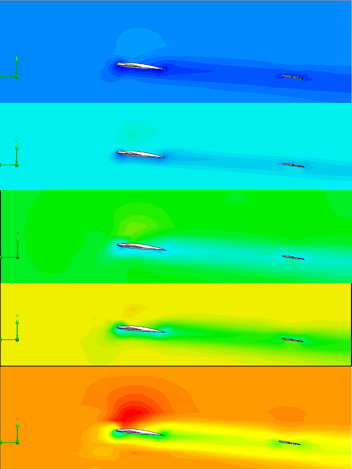
This plot is probably the most important to understand the behaviour of the Fox. the more we go down in the figures the more we increase the speed of entry of the air. we thus observe an evolution of the pressure and velocity fields. It seemed important to me to report the cut plots at the same scale to really observe the evolution of the phenomena, otherwise we observe the same thing at any speed of entry and the legend changes.

First of all, let's look at the graphs on the left. We observe at any speed that the flow passing above is faster than the reference speed. It is even more striking for the flow passing under the wing which is slower than the initial speed. This behaviour is vital to exert the lift. The most important is to notice that the more the entry speed is important, the wider the speed gradient is (very low speed below and very high speed above) for example at 25 m/s we have a gradient going from red to green (about 14 m/s difference) while at 5 m/s the gradient goes from dark blue to light blue (about 4 m/s difference)

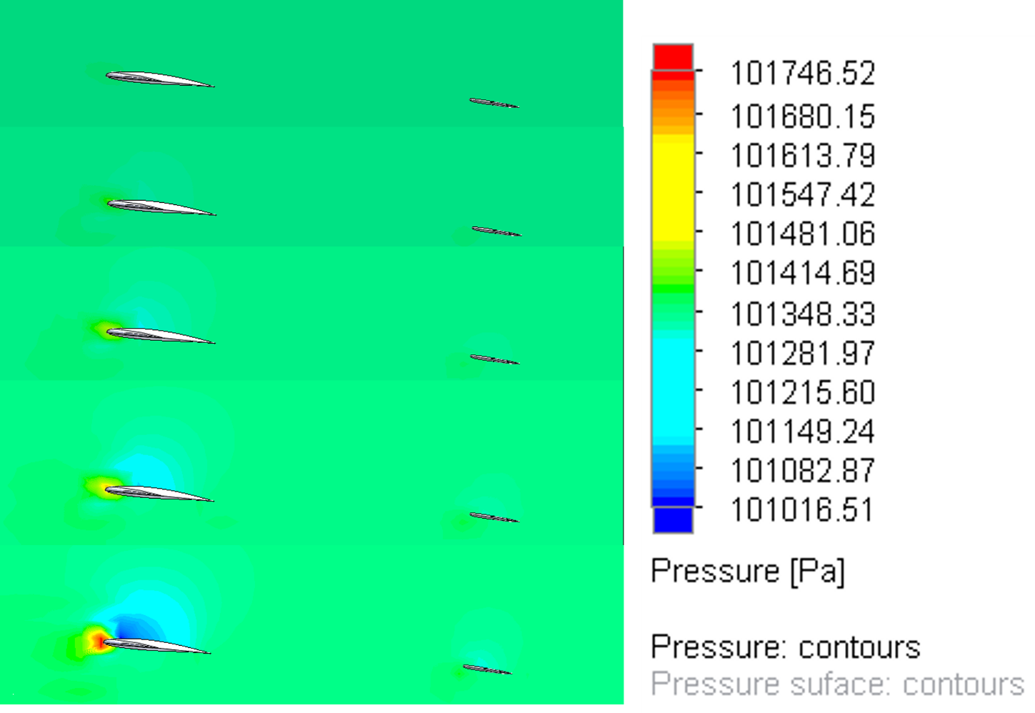
If we look at the pressure now, we can observe a pressure gradient at 15 m/s.

The behaviour of the wing is as follows, an important pressure is made on the leading edge, the air comes in pressure on this one then divides in 2 flows. The upper one going faster as seen previously, it creates a depression above the wing, it is the lift. In our case we notice that the wing has lift. The last point to raise is that it is logical that the minimum and maximum are calculated on the simulation at 25 m/s . The lift is in major part due to the foil shape and the angle of attack.

Input air (m.s^-1)

Air Velocity (m.s^-1)

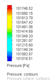
Pressure (Pa)

Scale

Scale

5

10

15

20

25

Table 1 : Comparison of Speed/Pressure fields as a function of aircraft speed

Table 2 : Comparison of Speed/Pressure fields as a function of aircraft speed

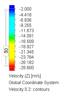
here we can observe different cut plot at 0.2, 1 and 2 meters of distance from the marker along the wing to observe the evolution of the behavior according to place on the wing

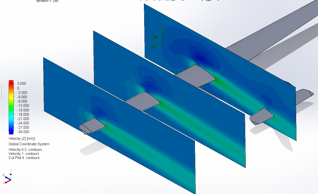
Figure 21 : airflow as a function of distance on the wing Fox

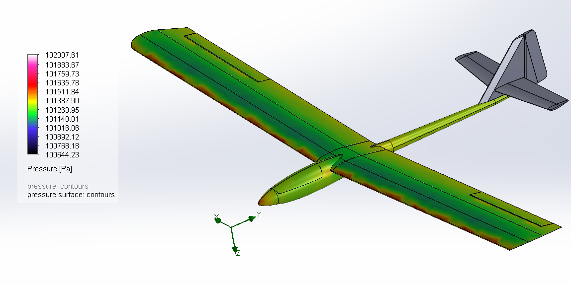
On the left is a surface plot to understand the pressure distribution on the aircraft. The blue band is the wing depression, the lift.

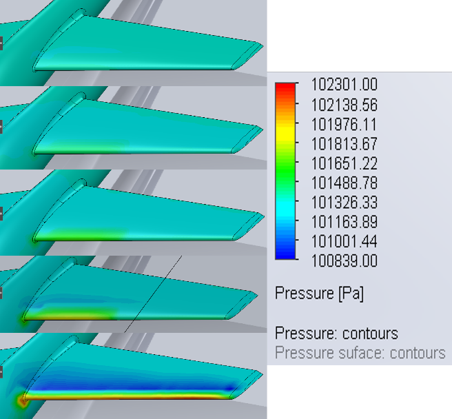
Figure 22 : Surface Pressure according to drone speed : Fox

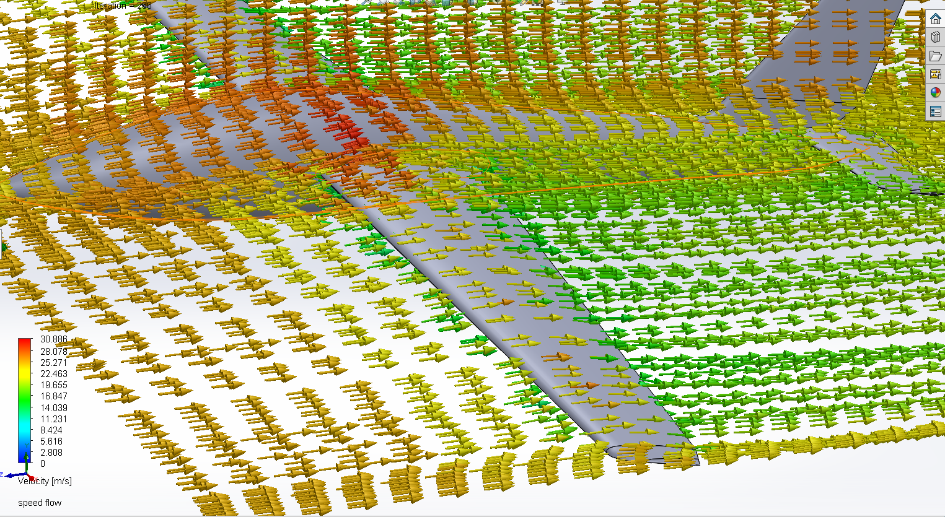
To finish with the qualitative analysis of the results here we have a flow trajectory plot where we can see the direction of the air and its speed in colour. We can see that the speed above is more important than below.

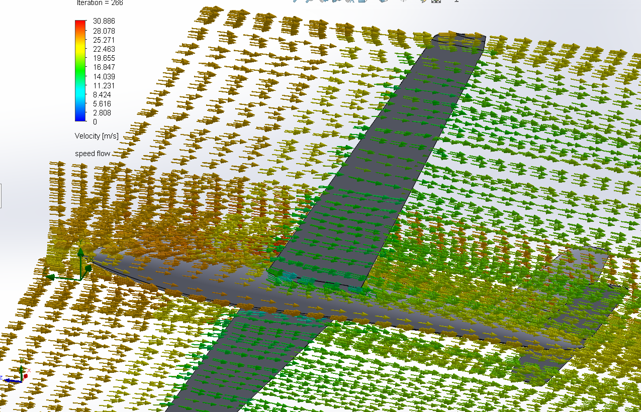
Figure 23 : Flow trajectory representing velocity Fox

Figure 24 : Flow trajectory representing velocity Fox

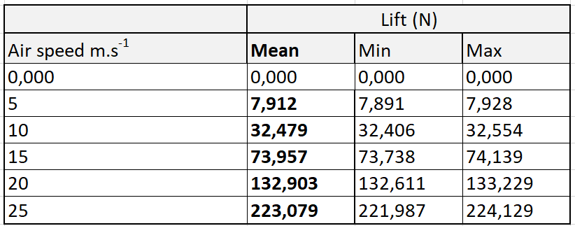Then we extract the goal data that we have chosen to focus mainly on the average lift of all the simulations see table 3. Then we put them in form, and we find a polynomial fit to characterize the behaviour of the Take Off.

Table 3 : Min, Max and Mean Lift for the Fox

To know how much lift, we need to take off, it's simple:

We know that the plane is 12 kg, to have the force of gravitation we make this calculation:

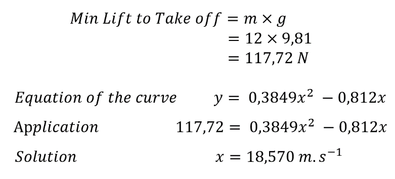
Equation 1 : Lift to take off Fox

Seagull behaviour

Now the analysis of the seagull is almost the same as the fox, we will skip the details

It should be noted that the simulation of the seagull was performed only on the blue areas including the nose of the aircraft. The empennage was excluded because it presented geometrical defaults.

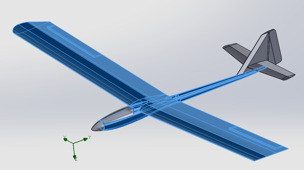
Figure 25 : objects included in the simulation

On this aircraft the lift is present as seen on the pressure and velocity cut plot

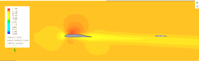
Figure 26 : Air Velocity cut plot (25 m.s^-1) Seagull

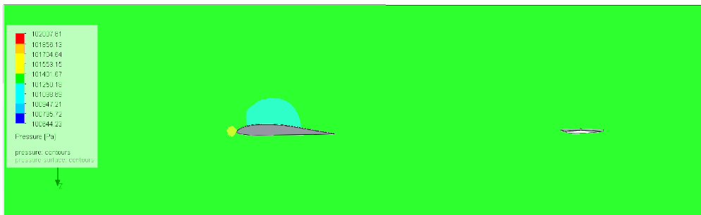
Figure 27 : Pressure Cut plot Seagull (25 m.s^-1)

The analysis is the same here, we observe a band of depression on the front top of the wing and the flow is faster above

Figure 28 : Surface pressure Seagull

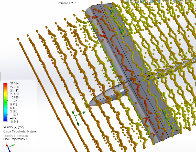
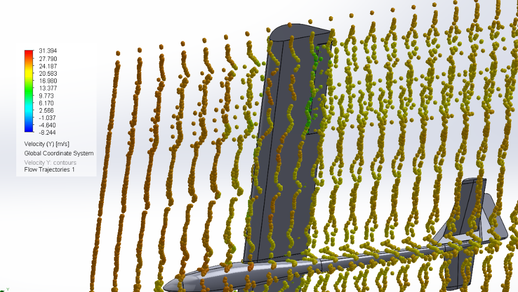
Figure 29 : Flow trajectory representing velocity Seagull

Figure 30 : Flow trajectory representing velocity Seagull

Here we apply exactly the same analysis as for the Fox

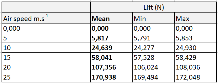
Table 4 : Min, Max and Mean Lift for the seagull

Table 5 : Min, Max and Mean of the Lift for the seagull

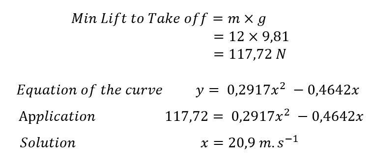
Equation 2 : Lift to take off Seagull

Comparison

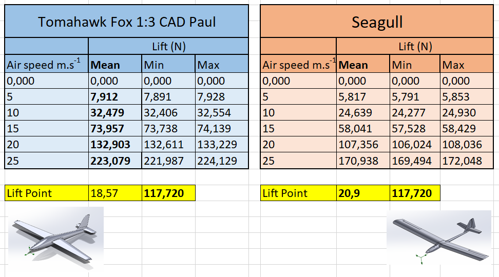
Figure 31 : Comparison between fox and seagull behaviour

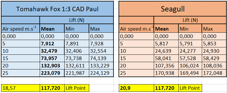
Table 6 : Fox/Seagull take off Comparison

By seeing these results side by side, we can conclude that

For the same acceleration the fox will take off earlier than the seagull. It has best properties.

Material matrix decision

Tableau 7 : Matrix decision between CFRP and GFRP for a fuselage

References

[1] https://www.differencebetween.com/difference-between-cfrp-and-gfrp/

[2] https://fr.strephonsays.com/cfrp-and-gfrp-11786

[3] https://aviation.stackexchange.com/questions/43298/how-do-gfrp-and-cfrp-compare

Hermansson, F. et al. (2022) ‘Can carbon fiber composites have a lower environmental impact than fiberglass?’, Resources, Conservation and Recycling, 181, p. 106234. Available at: https://doi.org/10.1016/j.resconrec.2022.106234.

Kim, J. et al. (2022) ‘Bond Strength Properties of GFRP and CFRP according to Concrete Strength’, Applied Sciences, 12(20), p. 10611. Available at: https://doi.org/10.3390/app122010611.

Annexes

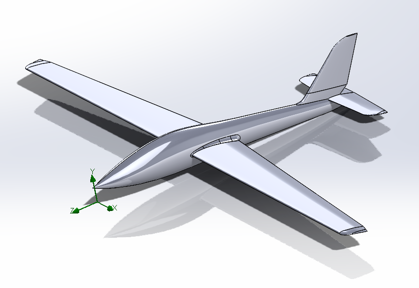
Figure : Global view Fox

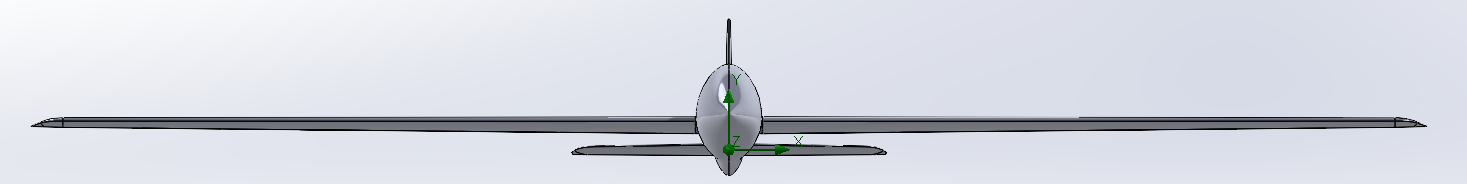
Figure : Front view Fox

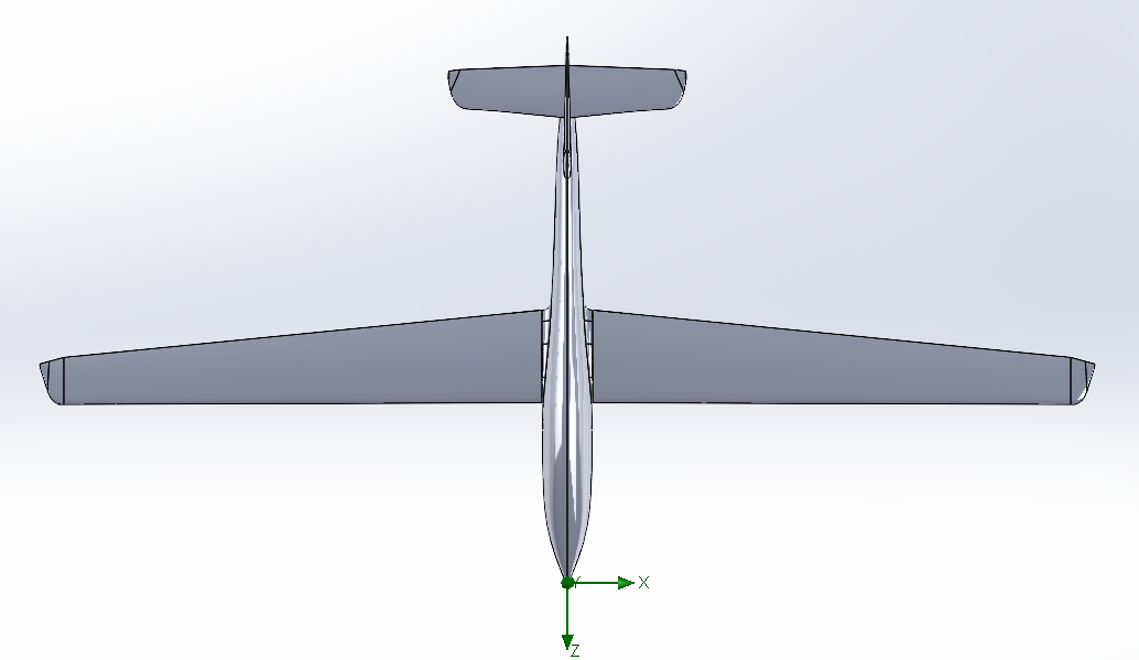
Figure : Top view Fox

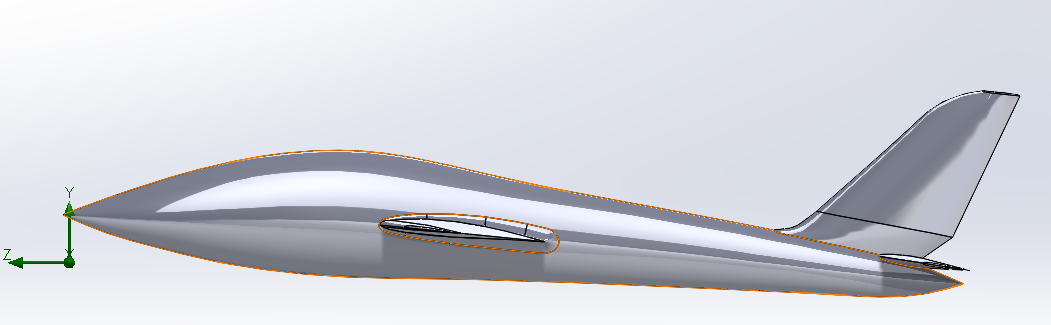
Figure : Right view Fox

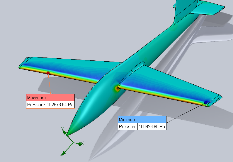
Figure 36 : Surface plot representing the field pressure, max and min value

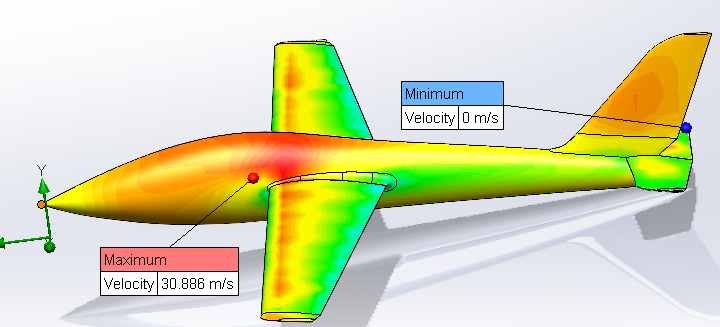
Figure 37 : Surface plot representing the field velocity, max and min value (Top of the wing)

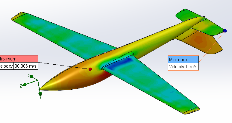
Figure 38 : Surface plot representing the field velocity, max and min value (Below the wing)

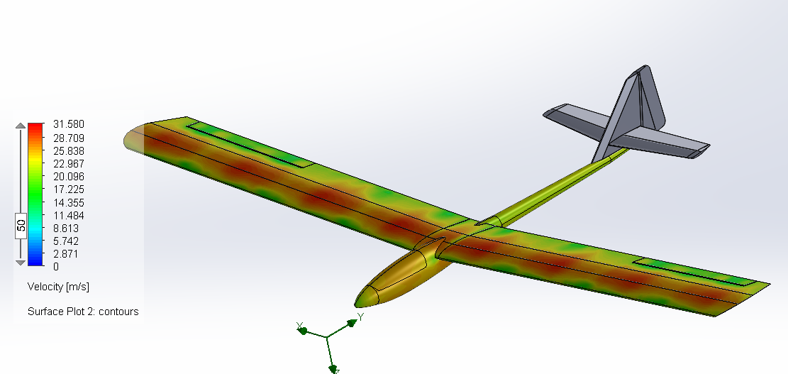
Figure 39 : Surface plot representing the field velocity Seagull