• Lexical (the text is viewed as a sequence of tokens grouped into sentences, with each token corresponding to a word, number, or punctuation mark):
  • Token-based (e.g., word length, sentence length, etc.);
  • Vocabulary richness (i.e., attempts to quantify the vocabulary diversity of a text);
  • Word frequencies (e.g., the traditional “bag-of-words” representation [21] in which texts become vectors of word frequencies disregarding contextual information, i.e., the word order);
  • Word n-grams (i.e., sequences of n contiguous words also known as word collocations);
  • Errors (i.e., intended to capture the idiosyncrasies of an author’s style) (requires orthographic spell checker).
• Character (the text is viewed as a sequence of characters):
  • Character types (e.g., letters, digits, etc.) (requires character dictionary);
  • Character n-grams (i.e., considers all sequences of n consecutive characters in the texts; n can have a variable or fixed length);
  • Compression methods (i.e., the use of a compression model acquired from one text to compress another text; compression models are usually based on repetitions of character sequences).
• Syntactic (text-representation which considers syntactic information):
  • Part-of-speech (POS) (requires POS tagger—a tool that assigns a tag of morpho-syntactic information to each word-token based on contextual information);
  • Chunks (i.e., phrases);
  • Sentence and phrase structure (i.e., a parse tree of each sentence is produced);
  • Rewrite rules frequencies (these rules express part of the syntactic analysis, helping to determine the syntactic class of each word as the same word can have different syntactic values based on different contexts);
  • Errors (e.g., sentence fragments, run-on sentences, mismatched use of tenses) (requires syntactic spell checker).
• Semantic (text-representation which considers semantic information):
  • Synonyms (requires thesaurus);
  • Semantic dependencies.
• Application-specific (the text is viewed from an application-specific perspective to better represent the nuances of style in a given domain):
  • Functional (requires specialized dictionaries);
  • Structural (e.g., the use of greetings and farewells in messages, types of signatures, use of indentation, and paragraph length);
  • Content-specific (e.g., content-specific keywords);
  • Language-specific.

• Instance-based approach (i.e., each training text is individually represented as a separate instance in the training process to create a reliable attribution model);
• Profile-based approach (i.e., a cumulative representation of an author’s style, also known as the author’s profile, is extracted by concatenating all available training texts of one author into one large file to flatten differences between texts).

2.2. Datasets

Table 1. Datasets used for author attribution detection; Author(s) are names of individuals who created the dataset (for a group consisting of more than two, only the name of the first person is provided in the list, followed by “et al.”); Paper is the first paper that introduced that dataset or that is recommended by its creator(s) to be used for citing the dataset; Language is the language in which the texts in the database were written; Size is the dimension of the dataset; Features stands for the types of features that can be or were used on that specific dataset (however, the information here is only indicative and should not be taken literally); No. of features, is also more an indicative value for possible feature set dimensions; Name or link provides the name by which that specific dataset is known and, when available, links are provided.

2.3. Strategies

2.4. Comparison

Table 2. State of the art macro-accuracy of authorship attribution models. Information collected from [10] (Tables 1 and 3). Name is the name of the dataset; No. docs represents the number of documents in that dataset; No. auth represents the number of authors; Content indicates whether the documents are cross-topic ( ) or cross-genre ( ); W/D stands for words per document, representing the average length of documents; imb represents the imbalance of the dataset measured by the standard deviation of the number of documents per author.

3. Proposed Dataset

The texts considered are Romanian stories, short stories, fairy tales, novels, articles, and sketches.

There are 400 such texts of different lengths, ranging from 91 to 39,195 words. Table 3 presents the averages and standard deviations of the number of words, unique words, and the ratio of words to unique words for each author. There are differences up to almost 7000 words between the average word counts (e.g., between Slavici and Oltean). For unique words, the difference between averages goes up to more than 1300 unique words (e.g., between Eminescu and Oltean). Even the ratio of total words to unique words is a significant difference between the authors (e.g., between Slavici and Oltean).

Table 3. Diversity of the considered dataset in terms of the length of the texts (i.e., number of words). Author is the author’s name (the last name is in bold); Average is the mean number of words per text written by the corresponding author; StdDev is the standard deviation; Average-Unique is the mean number of unique words; StdDev-Unique is the standard deviation on unique words; Average-Ratio is the mean number of the ratio of total words to unique words; StdDev-Ratio is the standard deviation of the ratio of total words to unique words.

Eminescu and Slavici, the two authors with the largest averages also have large standard deviations for the number of words and the number of unique words. This means that their texts range from very short to very long. Gârleanu and Oltean have the shortest texts, as their average number of words and unique words and the corresponding standard deviations are the smallest.

There is also a correlation between the three groups of values (pertaining to the words, unique words, and the ratio between the two) that is to be expected as a larger or smaller number of words would contain a similar proportion of unique words or the ratio of the two, while the standard deviations of the ratio of total words to unique words tend to be more similar. However, Slavici has a very high ratio, which means that there are texts in which he repeats the same words more often, and in other texts, he does not. There is also a difference between Slavici and Eminescu here because even if they have similar word count average and unique word count average, their ratio differs. Eminescu has a similar representation in terms of ratio and standard deviation with his lifelong friend Creangă, which can mean that both may have similar tendencies in reusing words.

Table 4 shows the averages of the number of features that are contained in the texts corresponding to each author. The pattern depicted here is similar to that in Table 3, which is to be expected. However, standard deviations tend to be similar for all authors. These standard deviations are considerable in size, being on average as follows:

Table 4. Diversity of the considered dataset in terms of the number of occurrences of the considered features in the texts. Author is the author’s name (the last name is in bold); Average-P is the average number of the occurrence of the considered prepositions in the texts corresponding to each author; StdDev-P is the standard deviation for the occurrence of the prepositions; Average-PA is the average number of the occurrence of the considered prepositions and adverbs; StdDev-PA is the standard deviation of the number of the occurrence of the considered prepositions and adverbs; Average-PAC is the average number of the occurrence of the considered prepositions, adverbs, and conjunctions; StdDev-PAC is the standard deviation of the number of the occurrence of the considered prepositions, adverbs, and conjunctions.

• 4.16 on the set of 56 features (i.e., the list of prepositions),
• 23.88 on the set of 415 features (i.e., the list of prepositions and adverbs),
• 25.38 on the set of 432 features (i.e., the list of prepositions, adverbs, and conjunctions).

This means that the frequency of feature occurrence differs even in the texts written by the same author.

The considered texts are collected from 4 websites and are written by 10 different authors, as shown in Table 5. The diversity of sources is relevant from a twofold perspective. First, especially for old texts, it is difficult to find or determine which is the original version. Second, there may be differences between versions of the same text either because some words are no longer used or have changed their meaning, or because fragments of the text may be added or subtracted. For some authors, texts are sourced from multiple websites.

Table 5. List of authors (the author’s last name is in bold), the number of texts considered for each author (total number is in bold), and their source (i.e., the website from which they were collected).

The diversity of the texts is intentional because we wanted to emulate a more likely scenario where all these characteristics might not be controlled. This is because, for future texts to be tested on the trained models, the text length, the source, and the type of writing cannot be controlled or imposed.

To highlight the differences between the time frames of the periods in which the authors lived and wrote the considered texts, as well as the environment from which the texts were intended to be read, we gathered the information presented in Table 6. It can be seen that the considered texts were written in the time span of three centuries. This also brings an increased diversity between texts, since within such a large time span there have been significant developments in terms of language (e.g., diachronic developments), writing style relating to the desired reading medium (e.g., paper or online), topics (e.g., general concerns and concerns that relate to a particular time), and viewpoints (e.g., a particular worldview).

Table 6. List of authors, time spans of the periods in which the authors lived and wrote the considered texts and the medium from which the readers read their texts. Author is the author’s name (the last name is in bold); Life is the lifetime of the author; Publication is the publication interval of the texts (note: the information presented here was not always easily accessible and some sources would contradict in terms of specific years, however, this information should be considered more as an indicative coordinate and should not be taken literally, the goal being that the literary texts be temporally framed in order to have a perspective on the period in which they were written/published); Century is a coarser temporal framing of the periods in which the texts were written; Medium is the environment from which most of the readers read the author’s texts.

The diversity of the texts also pertains to the type of writing, i.e., stories, short stories, fairy tales, novels, articles, and sketches. Table 7 shows the distribution of these types of writing among the texts belonging to the 10 authors. The difference in the type of writing has an impact on the length of the texts (for example, a novel is considerably longer than a short story), genre (for example, fairy tales have more allegorical worlds that can require a specific style of writing), the topic (for example, an article may describe more mundane topics, requiring a different type of discourse compared to the other types of writing).

Table 7. List of authors and types of writing of the considered texts. Author is the author’s name (the last name is in bold); Article include, in addition to articles written for various newspapers and magazines, other types of writing that did not fit into the other categories, but relate to this category, such as prose, essays, and theatrical or musical chronicles. Total number of texts per type are in bold.

Regarding the list of possible features, we selected as elements to identify the author of a text inflexible parts of speech (IPoS) (i.e., those that do not change their form in the context of communication): conjunctions, prepositions, interjections, and adverbs. Of these, we only considered those that were single-word and we removed the words that may represent other parts of speech, as some of them may have different functions depending on the context, and we did not use any syntactic or semantic processing of the text to carry out such an investigation.

We collected a list of 24 conjunctions that we checked on dexonline.ro (i.e., site that contains explanatory dictionaries of the Romanian language) not to be any other part of speech (not even among the inflexible ones). We also considered 3 short forms, thus arriving at a list of 27 conjunctions. The process of selecting prepositions was similar to that of selecting conjunctions, resulting in a list of 85 (including some short forms).

The lists of interjections and adverbs were taken from:

• https://ro.wiktionary.org/wiki/Categorie:Interjec%C8%9Bii_%C3%AEn_rom%C3%A2n%C4%83, accessed on 20 October 2022
• https://ro.wiktionary.org/wiki/Categorie:Adverbe_%C3%AEn_rom%C3%A2n%C4%83, accessed on 20 October 2022

To compile the lists of interjections and adverbs, we again considered only single-word ones and we eliminated words that may represent other parts of speech (e.g., proper nouns, nouns, adjectives, verbs), resulting in lists of 290 interjections and 670 adverbs.

The lists of the aforementioned IPoS also contain archaic forms in order to better identify the author. This is an important aspect that has to be taken into consideration (especially for our dataset which contains texts that were written over a time span of 3 centuries), as language is something that evolves and some words change as form and sometimes even as meaning or the way they are used.

From the lists corresponding to the considered IPoS features, we use only those that appear in the texts. Therefore, the actual lists of prepositions, adverbs, and conjunctions may be shorter. Details of the texts and the lists of inflexible parts of speech used can be found at reference [68].

4. Compared Methods

Below we present the methods we will use in our investigations.

4.1. Artificial Neural Networks

Artificial neural networks (ANN) is a machine learning method that applies the principle function approximation through learning by example (or based on provided training information) [69]. An ANN contains artificial neurons (or processing elements), organized in layers and connected by weighted arcs. The learning process takes place by adjusting the weights during the training process so that based on the input dataset the output outcome is obtained. Initially, these weights are chosen randomly.

The artificial neural structure is feedforward and has at least three layers: input, hidden (one or more), and output.

The experiments in this paper were performed using fast artificial neural network (FANN) [70] library. The error is RMSE. For the test set, the number of incorrectly classified items is also calculated.

4.2. Multi-Expression Programming

Multi-expression programming (MEP) is an evolutionary algorithm for generating computer programs. It can be applied to symbolic regression, time-series, and classification problems [71]. It is inspired by genetic programming [72] and uses three-address code [73] for the representation of programs.

MEP experiments use the MEPX software [74].

4.3. K-Nearest Neighbors

K-nearest neighbors (k-NN) [75,76,77] is a simple classification method based on the concept of instance-based learning [78]. It finds the k items, in the training set, that are closest to the test item and assigns the latter to the class that is most prevalent among these k items found.

The source code of k-NN used in this paper is written by us and is available at https://github.com/sanda-avram/ROST-source-code, (accessed on 8 November 2022) along other scripts and programs we wrote to perform the tests.

4.4. Support Vector Machine

A support vector machine (SVM) [79] is also a classification principle based on machine learning with the maximization (support) of separating distance/margin (vector). As in k-NN, SVM represents the items as points in a high-dimensional space and tries to separate them using a hyperplane. The particularity of SVM lies in the way in which such a hyperplane is selected, i.e., selecting the hyperplane that has the maximum distance to any item.

LIBSVM [80,81] is the support vector machine library that we used in our experiments. It supports classification, regression, and distribution estimation.

4.5. Decision Trees with C5.0

Classification can be completed by representing the acquired knowledge as decision trees [82]. A decision tree is a directed graph in which all nodes (except the root) have exactly one incoming edge. The root node has no incoming edge. All nodes that have outgoing edges are called internal (or test) nodes. All other nodes are called leaves (or decision) nodes. Such trees are built starting from the root by top–down inductive inference based on the values of the items in the training set. So, within each internal node, the instance space is divided into two or more sub-spaces based on the input attribute values. An internal node may consider a single attribute. Each leaf is assigned to a class. Instances are classified by running them through the tree starting from the root to the leaves.

See5 and C5.0 [83] are data mining tools that produce classifiers expressed as either decision trees or rulesets, which we have used in our experiments.

5. Numerical Experiments

To prepare the dataset for the actual building of the classification model, the texts in the dataset were shuffled and divided into training (50%), validation (25%), and test (25%) sets, as detailed in Table 8. In cases where we only needed training and test sets, we concatenated the validation set to the training set. We reiterated the process (i.e., shuffle and split 50%–25%–25%) three times and, thus, obtained three different training–validation–test shuffles from the considered dataset.

Table 8. List of authors (the author’s last name is in bold); the number of texts and their distribution on the training, validation, and test sets. The total number of texts per author, per set, and grand total are in bold.

Before building a numerical representation of the dataset as vectors of the frequency of occurrence of the considered features, we made a preliminary analysis to determine which of the inflexible parts of speech are more prevalent in our texts. Therefore, we counted the number of occurrences of each of them based on the lists described in Section 3. The findings are detailed in Table 9.

Table 9. The occurrence of inflexible parts of speech considered. IPoS stands for Inflexible part of speech; No. of occurrence is the total number of occurrences of the considered IPoS in all texts; % from total words represents the percentage corresponding to the No. of occurrence in terms of the total number of words in all texts (i.e., 1,342,133); No. of files represents the number of texts in which at least one word from the corresponding IPoS list appears; Avg. per file represents the No. of occurrence divided by the total number of texts/files (i.e., 400); and No. of IPoS represents the list length (i.e., the number of words) for each corresponding IPoS.

Based on the data presented here, we decided not to consider interjections because they do not appear in all files (i.e., 44 files do not contain any interjections), and in the other files, their occurrence is much less compared to the rest of the IPoS considered. This investigation also allowed us to decide the order in which these IPoS will be considered in our tests. Thus, the order of investigation is prepositions, adverbs, and conjunctions.

Therefore, we would first consider only prepositions, then add adverbs to this list, and finally add conjunctions as well. The process of shuffling and splitting the texts into training–validation–test sets (described at the beginning of the current section, i.e., Section 5) was reiterated once more for each feature list considered. We, therefore, obtained different dataset representations, which we will refer further as described in Table 10. The last 3 entries (i.e., ROST-PC-1, ROST-PC-2, and ROST-PC-3) were used in a single experiment.

Table 10. Names used in the rest of the paper refer to the different dataset representations and their shuffles. Only the first 9 entries (with the Designation written in bold) were used for the entire set of investigations.

Correspondingly, we created different representations of the dataset as vectors of the frequency of occurrence of the considered feature lists. All these representations (i.e., training-validation-test sets) can be found as text files at reference [68]. These files contain feature-based numerical value representations for a different text on each line. On the last column of these files, are numbers from 0 to 9 corresponding to the author, as specified in the first columns of Table 6, Table 7 and Table 8.

5.1. Results

The parameter setting for all 5 methods are presented in Appendix A, while Appendix B contains some prerequisite tests.

Most results are presented in a tabular format. The percentages contained in the cells under the columns named Best, Avg, or Error may be highlighted using bold text or gray background. In these cases, the percentages in bold represent the best individual results (i.e., obtained by the respective method on any ROST-*-* in the dataset, out of the 9 representations mentioned above), while the gray-colored cells contain the best overall results (i.e., compared to all methods on that specific ROST-X-n representation of the dataset).

5.1.1. ANN

Results that showed that ANN is a good candidate to solve this kind of problem and prerequisite tests that determined the best ANN configuration (i.e., number of neurons on the hidden layer) for each dataset representation are detailed in Appendix B.1. The best values obtained for test errors and the number of neurons on the hidden layer for which these “bests” occurred are given in Table 11. These results show that the best test error rates were mainly generated by ANNs that have a number of neurons between 27 and 49. The best test error rate obtained with this method was for ROST-PAC-3, while the best average was for ROST-PAC-2.

Table 11. ANN results on the considered datasets. On each set, 30 runs are performed by ANNs with the hidden layer containing from 5 to 50 neurons. The number of incorrectly classified data is given as a percentage (the best results obtained by ANN on any ROST-*-* dataset representation are in bold). Best stands for the best solution (out of 30 runs on each of the 46 ANNs), Avg stands for Average (over 30 runs), StdDev stands for Standard Deviation, and No. of neurons stands for the number of neurons in the hidden layer of the ANN that produced the best solution. The best result obtained by ANN compared to all methods for a given ROST-X-n dataset representation is in a gray cell.

5.1.2. MEP

Results that showed that MEP can handle this type of problem are described in Appendix B.2.

We are interested in the generalization ability of the method. For this purpose, we performed full (30) runs on all datasets. The results, on the test sets, are given in Table 12.

Table 12. MEP results on the considered datasets. A total of 30 runs are performed. The number of incorrectly classified data is given as a percentage (the best results obtained by MEP on any ROST-*-* dataset representation are in bold). Best stands for the best solution (out of 30 runs), Avg stands for Average (over 30 runs) and StdDev stands for Standard Deviation. The best result obtained by MEP compared to all methods for a given ROST-X-n dataset representation is in a gray cell.

With this method, we obtained an overall “best” on all ROST-*-*, which is , and also an overall “average” best with a value of , both for ROST-PA-2.

One big problem is overfitting. The error on the training set is low (they are not given here, but sometimes are below 10%). However, on the validation and test sets the errors are much higher (2 or 3 times higher). This means that the model suffers from overfitting and has poor generalization ability. This is a known problem in machine learning and is usually corrected by providing more data (for instance more texts for an author).

5.1.3. k-NN

Preliminary tests and their results for determining the best value of k for each dataset representation are presented in Appendix B.3.

The best k-NN results are given in Table 13 with the corresponding value of k for which these “bests” were obtained. It can be seen that for all ROST-P-*, the values of k were higher (i.e., ) than those for ROST-PA-* or ROST-PAC-* (i.e., ). The best value obtained by this method was for ROST-PAC-2 and ROST-PAC-3.

Table 13. k-NN results on the considered datasets. In total, 30 runs are performed with k varying with the run index. The number of incorrectly classified data is given as a percentage (the best results obtained by k-MM on any ROST-*-* dataset representation are in bold). Best stands for the best solution (out of the 30 runs), k stands for the value of k for which the best solution was obtained.

5.1.4. SVM

Prerequisite tests to determine the best kernel type and a good interval of values for the parameter are described in Appendix B.4, along with their results.

We ran tests for each kernel type and with nu varying from 0.1 to 1, as we saw in Figure A6 that for values less than 0.1, SVM is unlikely to produce the best results. The best results obtained are shown in Table 14.

Table 14. SVM results on the considered datasets. The number of incorrectly classified data is given as a percentage (the best results obtained by SVM on any ROST-*-* dataset representation are in bold). Best stands for the best test error rate (out of 30 runs with ranging from 0.001 to 1), and nu stands for the parameter specific to the selected type of SVM (i.e., nu-SVC). Results are given for each type of kernel that was used by the SVM. The best result obtained by SVM compared to all methods for a given ROST-X-n dataset representation is in a gray cell.

As can be seen, the best values were obtained for values of parameter nu between 0.2 and 0.6 (where sometimes 0.6 is the smallest value of the set {0.6, 0.7, ⋯, 1} for which the best test error was obtained). The best value obtained by this method was for ROST-PAC-1, using the linear kernel and nu parameter value 0.2.

5.1.5. Decision Trees with C5.0

Advanced pruning options for optimizing the decision trees with C5.0 model and their results are presented in Appendix B.5. The best results were obtained by using cases option, as detailed in Table 15.

Table 15. Decision tree results on the considered datasets. The number of incorrectly classified data is given as a percentage (the best results obtained by DT with C5.0 on any ROST-*-* dataset representation are in bold). Error stands for the test error rate, Size stands for the size of the decision tree required for that specific solution and cases stands for the threshold for which is decided to have two more that two branches at a specific branching point ( ). The best result obtained by DT with C5.0 compared to all methods for a given ROST-X-n dataset representation is in a gray cell.

The best result obtained by this method was on ROST-PAC-2, with 14 option, on a decision tree of size 12. When no options were used, the size of the decision trees was considerably larger for ROST-P-* (i.e., ≥57) than those for ROST-PA-* and ROST-PAC-* (i.e., ≤39).

5.2. Comparison and Discussion

The findings of our investigations allow for a twofold perspective. The first perspective refers to the evaluation of the performance of the five investigated methods, as well as to the observation of the ability of the considered feature sets to better represent the dataset for successful classification. The other perspective is to place our results in the context of other state-of-the-art investigations in the field of author attribution.

5.2.1. Comparing the Internally Investigated Methods

From all the results presented above, upon consulting the tables containing the best test error rates, and especially the gray-colored cells (which contain the best results while comparing the methods amongst themselves) we can highlight the following:

• ANN:

  -

  Four best results for: ROST-PA-1, ROST-PA-3, ROST-PAC-2 and ROST-PAC-3 (see Table 11);

  -

  Best ANN 23.46% on ROST-PAC-3; best ANN average 36.93% on ROST-PAC-2;

  -

  Worst best overall on ROST-P-1.

• MEP:

  -

  Two best results for ROST-PA-2 and ROST-PAC-3 (see Table 12);

  -

  Best overall 20.40% on ROST-PA-2; best overall average 27.95% on ROST-PA-2;

  -

  Worst best MEP on ROST-P-1.

• k-NN:

  -

  Zero best results (see Table 13);

  -

  Best k-NN 29.59% on ROST-PAC-2 and ROST-PAC-3;

  -

  Worst k-NN on ROST-P-2.

• SVM:

  -

  Four best results for: ROST-P-1, ROST-P-3, ROST-PAC-1 and ROST-PAC-2 (see Table 14);

  -

  Best SVM 23.44% on ROST-PAC-1;

  -

  Worst SVM on ROST-P-2.

• Decision trees:

  -

  Two best results for: ROST-P-2 and ROST-PAC-2 (see Table 15);

  -

  Best DT 24.5% on ROST-PAC-2;

  -

  Worst DT on ROST-P-2.

Other notes from the results are:

• Best values for each method were obtained for ROST-PA-2 or ROST-PAC-*;
• The worst of these best results were obtained for ROST-P-1 or ROST-P-2;
• ANN and MEP suffer from overfitting. The training errors are significantly smaller than the test errors. This problem can only be solved by adding more data to the training set.

An overview of the best test results obtained by all five methods is given in Table 16.

Table 16. Top of methods on each shuffle of each dataset, based on the best results achieved by each method. The gray-colored box represents the overall best (i.e., for all datasets and with all methods).

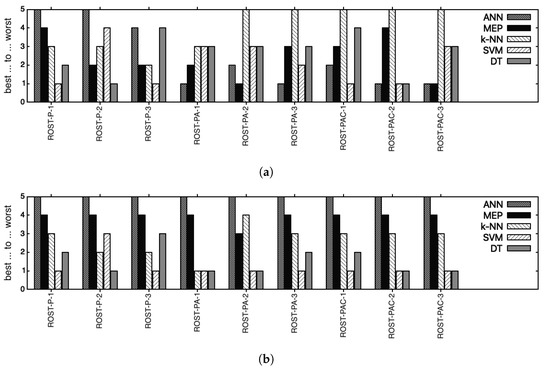
ANN ranks last for all ROST-P-* and ranks 1st and 2nd for ROST-PA-* and ROST-PAC-*. MEP is either ranked 1st or ranked 2nd on all ROST-*-* with three exceptions, i.e., for ROST-P-1 and ROST-PAC-2 (at 4th place) and for ROST-PAC-1 (at 3rd place). k-NN performs better (i.e., 3rd and 2nd places) on ROST-P-*, and ranks last for ROST-PA-* and ROST-PAC-*. SVM is ranked 1st for ROST-P-* and ROST-PAC-* with two exceptions: for ROST-P-2 (ranked 4th) and for ROST-PAC-3 (on 3rd place). For ROST-PA-* SVM is in 3rd and 2nd places. Decision trees (DT) with C5.0 is mainly on the 3rd and 4th places, with three exceptions: for ROST-P-1 (on 2nd place), for ROST-P-2 (on 1st place), and for ROST-PAC-2 (on 1st place).

An overview of the average test results obtained by all five methods is given in Table 17. However, for ANN and MEP alone, we could generate different results with the same parameters, based on different starting seed values, with which we ran 30 different runs. For the other 3 methods, we used the best results obtained with a specific set of parameters (as in Table 16).

Table 17. Top of methods on average results on each shuffle of each dataset. For k-NN, SVM, and DT we do not have 30 runs with the same parameters, so for these methods, the best values are presented here. The gray-colored box represents the overall best average (i.e., on all datasets and with all methods).

Comparing all 5 methods based on averages, SVM and DT take the lead as the two methods that share the 1st and 2nd places with two exceptions, i.e., for ROST-P-2 and ROST-P3 for which SVM and DT, respectively, rank 3rd. k-NN usually ranks 3rd, with four exceptions, when k-NN was ranked 2nd for ROST-P-2 and ROST-P-3, for ROST-PA-1 for which k-NN ranks 1st together with SVM and DT, and for ROST-PA-2 for which k-NN ranks 4th. MEP is generally ranked 4th with one exception, i.e., for ROST-PA-2 for which it ranks 3rd. ANN ranks last for all ROST-*-*.

For a better visual representation, we have plotted the results from Table 16 and Table 17 in Figure 1.

Figure 1. Top of methods on each shuffle of each dataset. Lower values are better. (a) Top of best results obtained by all methods (b) Top of average results, when applicable (i.e., over 30 runs for ANN and MEP).

We performed statistical tests to determine whether the results obtained by MEP and ANN are significantly different with a 95% confidence level. The tests were two-sample, equal variance, and two-tailed T-tests. The results are shown in Table 18.

Table 18. p-values obtained when comparing MEP and ANN results over 30 runs. No. of neurons used by ANN on the hidden layer represents the best-performing ANN structure on the specific ROST-*-*.

The p-values obtained show that the MEP and ANN test results are statistically significantly different for almost all ROST-*-* (i.e., ) with one exception, i.e., for ROST-PAC-2 for which the differences are not statistically significant (i.e., ).

Next, we wanted to see which feature set, out of the three we used, was the best for successful author attribution. Therefore, we plotted all best and best average results obtained with all methods (as presented in Table 16 and Table 17) on all ROST-*-* and aggregated on the three datasets corresponding to the distinct feature lists, in Figure 2.

Figure 2. Results on the best solutions obtained on the considered datasets. The percentage of incorrectly classified data is plotted. Best stands for the best solution, Avg stands for Average and the Standard Deviation is represented by error bars. (a) Best, Average and Standard Deviation are computed on the values from Table 16; (b) Best, Average, and Standard Deviation are computed on the values given in Table 17.

Based on the results represented in Figure 2a (i.e., which considered only the best results, as detailed in Table 16) we can conclude that we obtained the best results on ROST-PA-* (i.e., corresponding to the 415 feature set, which contains prepositions and adverbs). However, using the average results, as shown in Figure 2b and detailed in Table 17 we infer that the best performance is obtained on ROST-PAC-* (i.e., corresponding to the 432-feature set, containing prepositions, adverbs, and conjunctions).

Another aspect worth mentioning based on the graphs presented in Figure 2 is related to the standard deviation (represented as error bars) between the results obtained by all methods considered on all considered datasets. Standard deviations are the smallest in Figure 2a, especially for ROST-PA-* and even more so for ROST-PAC-*. This means that the methods perform similarly on those datasets. For ROST-P-* and in Figure 2b, the standard deviations are larger, which means that there are bigger differences between the methods.

5.2.2. Comparisons with Solutions Presented in Related Work

To better evaluate our results and to better understand the discriminating power of the best performing method (i.e., MEP on ROST-PA-2), we also calculate the macro-accuracy (or macro-average accuracy). This metric allows us to compare our results with the results obtained by other methods on other datasets, as detailed in Table 2. For this, we considered the test for which we obtained our best result with MEP, with a test error rate of 20.40%. This means that 20 out of 98 tests were misclassified.

To perform all the necessary calculations, we used the Accuracy evaluation tool available at [84], build based on the paper [85]. By inputting the vector of targets (i.e., authors/classes that were the actual authors (i.e., correct classifications) of the test texts) and the vector of outputs (i.e., authors/classes identified by the algorithm as the authors of the test texts), we were first given a Confusion value of and the Confusion Matrix, depicted in Table 19.

Table 19. Confusion Matrix (on the right side). Column headers and row headers (i.e., numbers from 0 to 9 that are written in bold) are the codes ¹ given to our authors, as specified on the left side.

This matrix is a representation that highlights for each class/author the true positives (i.e., the number of cases in which an author was correctly identified as the author of the text), the true negatives (i.e., the number of cases where an author was correctly identified as not being the author of the text), the false positives (i.e., the number of cases in which an author was incorrectly identified as being the author of the text), the false negatives (i.e., the number of cases where an author was incorrectly identified as not being the author of the text). For binary classification, these four categories are easy to identify. However, in a multiclass classification, the true positives are contained in the main diagonal cells corresponding to each author, but the other three categories are distributed according to the actual authorship attribution made by the algorithm.

For each class/author, various metrics are calculated based on the confusion matrix. They are:

• Precision—the number of correctly attributed authors divided by the number of instances when the algorithm identified the attribution as correct;
• Recall (Sensitivity)—the number of correctly attributed authors divided by the number of test texts belonging to that author;
• F-score—a combination of the Precision and Recall (Sensitivity).

Based on these individual values, the Accuracy Evaluation Results are calculated. The overall results are shown in Table 20.

Table 20. Accuracy evaluation Results. The macro-accuracy and corresponding macro-error are in bold.

Metrics marked with (Micro) are calculated by aggregating the contributions of all classes into the average metric. Thus, in a multiclass context, micro averages are preferred when there might be a class imbalance, as this method favors bigger classes. Metrics marked with (Macro) treat each class equally by averaging the individual metrics for each class.

Based on these results, we can state that the macro-accuracy obtained by MEP is 88.84%. We have 400 documents, and 10 authors in our dataset. The content of our texts is cross-genre (i.e., stories, short stories, fairy tales, novels, articles, and sketches) and cross-topic (as in different texts, different topics are covered). We also calculated an average number of words per document, which is 3355, and the imbalance (considered in [10] to be the standard deviation of the number of documents per author), which in our case is 10.45. Our type of investigation can be considered to be part of the Ngram class (this class and other investigation-type classes are presented in Section 2.4). Next, we recreated Table 2 (depicted in Section 2.4) while reordering the datasets based on their macro-accuracy results obtained by Ngram class methods in reverse order, and we have appropriately placed details of our own dataset and the macro-accuracy we achieved with MEP as shown above. This top is depicted in Table 21.

Table 21. State of the art macro-accuracy of authorship attribution models. Information collected from [10] (Tables 1 and 3). Name is the name of the dataset; No.docs represents the number of documents in that dataset; No. auth represents the number of authors; Content indicates whether the documents are cross-topic ( ) or cross-genre ( ); W/D stands for words per documents, being the average length of documents; imb represents the imbalance of the dataset as measured by the standard deviation of the number of documents per author.

We would like to underline the large imbalance of our dataset compared with the first two datasets, the fact that we had fewer documents, and the fact that the average number of words in our texts, although higher, has a large standard deviation, as already shown in Table 3. Furthermore, as already presented in Section 3, our dataset is by design very heterogeneous from multiple perspectives which are not only in terms of content and size, but also the differences that pertain to the time periods of authors, the medium they wrote for (paper or online media), and the sources of the texts. Although all these aspects do not restrict the new test texts to certain characteristics (to be easily classified by the trained model), they make the classification problem even harder.

6. Conclusions and Further Work

In this paper, we introduced a new dataset of Romanian texts by different authors. This dataset is heterogeneous from multiple perspectives, such as the length of the texts, the sources from which they were collected, the time period in which the authors lived and wrote these texts, the intended reading medium (i.e., paper or online), and the type of writing (i.e., stories, short stories, fairy tales, novels, literary articles, and sketches). By choosing these very diverse texts we wanted to make sure that the new texts do not have to be restricted by these constraints. As features, we wanted to use the inflexible parts of speech (i.e., those that do not change their form in the context of communication): conjunctions, prepositions, interjections, and adverbs. After a closer investigation of their relevance to our dataset, we decided to use only prepositions, adverbs, and conjunctions, in that specific order, thus having three different feature lists of (1) 56 prepositions; (2) 415 prepositions and adverbs; and (3) 432 prepositions, adverbs, and conjunctions. Using these features, we constructed a numerical representation of our texts as vectors containing the frequencies of occurrence of the features in the considered texts, thus obtaining 3 distinct representations of our initial dataset. We divided the texts into training–validation–test sets of 50%–25%–25% ratios, while randomly shuffling them three times in order to have three randomly selected arrangements of texts in each set of training, validation, and testing.

To build our classifiers, we used five artificial intelligence techniques, namely artificial neural networks (ANN), multi-expression programming (MEP), k-nearest neighbor (k-NN), support vector machine (SVM), and decision trees (DT) with C5.0. We used the trained classifiers for authorship attribution on the texts selected for the test set. The best result we obtained was with MEP. By using this method, we obtained an overall “best” on all shuffles and all methods, which is of a error rate.

Based on the results, we tried to determine which of the three distinct feature lists lead to the best performance. This inquiry was twofold. First, we considered the best results obtained by all methods. From this perspective, we achieved the best performance when using ROST-PA-* (i.e., the dataset with 415 features, which contains prepositions and adverbs). Second, we considered the average results over 30 different runs for ANN and MEP. These results indicate that the best performance was achieved when using ROST-PAC-* (i.e., the dataset with 432 features, which contains prepositions, adverbs, and conjunctions).

We also calculated the macro-accuracy for the best MEP result to compare it with other state-of-the-art methods on other datasets.

Given all the trained models that we obtained, the first future work is using ensemble decision. Additionally, determining whether multiple classifiers made the same error (i.e., attributing one text to the same incorrect author instead of the correct one) may mean that two authors have a similar style. This investigation can also go in the direction of detecting style similarities or grouping authors into style classes based on such similarities.

Extending our area of research is also how we would like to continue our investigations. We will not only fine-tune the current methods but also expand to the use of recurrent neural networks (RNN) and convolutional neural networks (CNN).

Regarding fine-tuning, we have already started an investigation using the top N most frequently used words in our corpus. Even though we have some preliminary results, this investigation is still a work in progress.

Using deep learning to fine-tune ANN is another direction we would like to tackle. We would also like to address overfitting and find solutions to mitigate this problem.

Linguistic analysis could help us as a complementary tool for detecting peculiarities that pertain to a specific author. For that, we will consider using long short-term memory (LSTM) architectures and pre-trained BERT models that are already available for Romanian. However, considering that a large section of our texts was written one or two centuries ago, we might need to further train BERT to be able to use it in our texts. That was one reason that we used inflexible parts of speech, as the impact of the diachronic developments of the language was greatly reduced.

We would also investigate the profile-based approach, where texts are treated cumulatively (per author) to build a profile, which is a representation of the author’s style. Up to this point we have treated the training texts individually, an approach called instance-based.

In terms of moving towards other types of neural networks, we would like to achieve the initial idea from which this entire area of research was born, namely finding a “fingerprint” of an author. We already have some incipient ideas on how these instruments may help us in our endeavor, but these new directions are still in the very early stages for us.

Improving upon the dataset is also high on our priority list. We are considering adding new texts and new authors.