Electroencephalography (EEG) in brain-computer interface (BCI) applications is often used compared to other modes such as functional magnetic resonance imaging (fMRI), functional near-infrared spectroscopy (fNIRS), and its low cost and quick response time [1]. Most BCI signals work well from certain places on the scalp. On the contrary, noisy and redundant signals can degrade the BCI efficiency [2,3,4,5,6]. Furthermore, using high channels requires a lengthy preparation time, impacting BCI’s usability. Consequently, picking the fewest channel numbers while maintaining maximum or required accuracy will help to achieve both efficiency and ease. However, identifying the appropriate channel selection is not easy, as manually selecting channels based on neuroscientific data does not always give optimal results compared to using all EEG channels [2].

A brain-computer interface aims to convert basic cerebral information into motor commands that a neuroprosthetic device can replicate. Kinesthetic and visual motor imagery (KMI and VMI) are the two basic categories of motor imagery [7]. KMI is characterized by the ability to simulate a movement by creating an impression of how muscles contract and feel during a actual movement. On the other hand, the capacity to see oneself doing the movement is known as VMI. KMI could be more efficient than VMI since most decoders for motor prediction are created based on actual movement. Therefore, employing a KMI to enhance the BCI performance would be preferable. However, individuals could become confused about the visual techniques without explicit instructions. Furthermore, people with motor disabilities had more difficulty using kinesthetic imagery than healthy people [8]. One could categorize the various visual kinds and provide the subject with feedback. With the motor imagery (MI) EEG data, many EEG channel selection algorithms have been developed since 2010 [9,10]. The study of movement and imagery-related activity revealed broadly dispersed frontoparietal cortical regions, the medical aspect of the superior frontal gyrus, the the anterior cingulate cortex, frontal and temporal opercular areas, occipital areas, and the posterolateral cerebellum. In an earlier trial with the sequential movement and imagery (SMI) task, this activity pattern was identical to the usual movement and image activity [11]. As a result, frequency-specific variations in a continuous EEG are event-related phenomena [12].

According to studies, the user’s MI stimulates the sensory-motor cortex in the brain, increasing metabolism and blood flow while decreasing or blocking the amplitude of μ (8–13 Hz) and β (14–30 Hz) rhythm EEG signals and oscillation frequency. This is referred to as ERD. On another side of the phenomenon called “event-related synchronization” (ERS), the amplitude of μ rhythm and the β rhythm of EEG signal increases.

Subjective consciousness elicits MI-based EEG, an endogenous evoked activity [33]. It depicts the dynamic process of emotional thought from conception to completion. Similarly, related research in sports rehabilitation suggests that MI training can aid in nerve healing and regeneration of motor nerve routes. As a result, investigating MI-based EEG signals’ processing and use are critical. The difficulty is that EEG and physiological phenomena are more complex than absolute motion, making them harder to detect and treat.

Two crucial phases in EEG signal analysis are EEG pre-processing and feature extraction. Pre-processing techniques aid in the removal of undesirable artifacts from the EEG signal, improving the signal-to-noise ratio. By isolating the noise from the actual signal, a pre-processing block aids in increasing the system’s performance. Following that, a feature extraction block aids in retrieving the signal’s most essential features. These characteristics will help the decision-making mechanism get the intended result.

The electroencephalogram (EEG) helps detect brain activity and behavior. However, artifacts in the recorded electrical activity will always impact the processing of the EEG data. As a result, developing ways to recognize and extract clean EEG data during encephalogram recordings is critical. Several approaches for removing artifacts have been proposed. However, artifact removal research remains a work in progress [34].

Because EEG signal-gathering equipment is now widely available, BCI based on EEG has become a popular subject for study in recent decades. Since we can capture brain activity data with many channels, EEG equipment is cost-effective compared to other approaches. Researchers can create ways to identify the best channels because there are so many of them. These algorithms are intended to reduce the calculation time, increase classification accuracy, and select the best channels for a specific application or activity. 

The EEG channel selection methods were taken from feature selection algorithms published in the literature. Feature selection chooses the best subset of features, whereas channel selection employs these methods to choose a channel. After selecting the best channel set, the features are extracted for categorization. On the other hand, the best feature set is fed straight to the classification algorithm in feature selection. The collected features of an optimum channel subset cannot produce good results when selecting a filter channel. To evaluate the credibility of a feature subset, a criterion is used. Since the number of functions is similar to the size of the signal, larger signals have more features. The discovery of an optimal subset is a complicated problem called the non-deterministic polynomial-time (NP) [35].

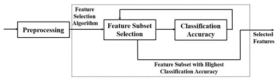
As illustrated in Figure 1, most feature selection methods have two steps. A heuristic search strategy such as full search, random search, or sequential search is employed to select assessment features during the sub-set production stage correctly. Each new subset of applicant features is reviewed, and its results are compared to the first-best, depending on the classification accuracy.

If the newly selected features outperform the prior one, the new contender will be promoted to the position of the previously selected feature. The process of producing and assessing features is continued until a stop criterion is fulfilled.

This section gives a brief introduction to CSP methods.

The classical CSP diagonalizes the two covariance matrices concurrently [36]. Let X∈R^M×N denote a matrix of EEG signals that have been observed, where the channel number is M and the samples are denoted by N. The classic CSP problem is stated as follows: where w is a spatial filter coefficient, Ci(i=1,2) indicates a single-class covariance matrix. Generally, the generalised eigenvalue decomposition (EVD) can handle this problem. where λ is an eigenvalue of C1 and C2. Moreover, M eigenvectors are generalizations obtained by solving Equation (2). In practice, one use the first r eigenvectors {wi}ri=1 and the last eigenvectors r and {wi}ri=M−r+1 as spatial filters, if the eigenvalues {λi}Mi=1. They are organized according to their size in a non-ascending way. We ultimately define W=[w1,…,wr,wM−r+1,…,wM]. These issues led to the choice to spread the spatial filters of the CSP, focusing on a few channels with significant class variations and avoiding channels with low or irregular noise or artifact variations. The rows of the CSP projection matrix assigns uniform channel weights to maximize discrepancies between two EEG signal types. Therefore, the vectors of the source distribution can be considered the CSP space filters.

Due to classic CSP inadequacies, several researchers aim to integrate sparsing behavior with conventional CSP to discover and eliminate highly noisy or interfering channels. Given w’s sparsity k, i.e., the number of nonzero items in w. The sparse CSP problem is stated as follows:

The ∥.∥0 is the Euclidean distance and the problem can be converted into Equation (2) typical problems if k channels are specified. Where C1,k and C2,k are the k × k sub-matrices of C1 and C2. However, this is generally impractical. To tackle such a problem, further develop forward selection (F.S.), reverse elimination (R.E.), and recursive weight removal (RWE) [37].

A regularized CSP (RCSP) approach is recommended to regularize the covariance matrix estimate in CSP extraction. Regularized covariance-matrix estimation is employed in the Regularized CSP algorithm in RCSP by applying the regularization technique presented in the general learning concept [38,39]. The CSP algorithm is regulated in a small sample environment (SSS). There are two regularization parameters used in [38]. The first regularization parameter orients the reduction of a specific subject covariance matrix to a more general covariance matrix to lower the estimated variance. This is based on the [39]. The second parameter of regularization limits the reduction of the sample-based covariance estimate in the direction of a scaled identification matrix to the bias due to the restricted number of samples. In addition, the challenge of determining regularization parameters for RCSP must be solved. On the other hand, the number of samples in SSS may not be enough for regularization parameters to be determined by the approach, which is used commonly [38]. Consequently, the tensor object recognition aggregation technology is employed to identify the regularization parameters in the EEG signal classification using RCSP that aggregates various regularized CSPs to generate a solution based on an ensemble [40].

The study helps to choose highly corresponding EEG channels for each patient against one reference channel without affecting classification accuracy. An individual channel sub-set provides a more efficient classification while lowering the computing complexity and time.

Spectral entropy is a theoretically describable measure of signal disorder: the correlation coefficient of spectral entropy of motor imaging was employed to identify series channel groups. The Filter Bank Common Spatial Pattern (FBCSP) algorithm assessed the performance of the channel groups.

The probability is Ei, where E=E1,E2,…,EN is the signal in the P(Ei) time domain. The algorithm calculates the signal of each layer based on the autoregression model. This investigation uses the correlation coefficient approach to picking channels using the “interested class vs. the rest” strategy. EEG is divided into two groups, s1 and s2, which includes the s1 interest group. H1 and H2 are spectral entropy identified to match s1 and s2. “Spectropic entropy correlation” is the relationship between the two groups s1 and s2. This is a measure of how tightly these two groups, represented as where σH1 is the standard deviation of the spectral entropy, and j is the index of the channel. We calculate the spectral entropy for each channel in all frequency ranges for selection by employing a total square correlation coefficient. where a spectral entropy estimate of i=1,2,…,N is the number of frequency bins. The channels are chosen based on the channels’ ρ(H1,j,H2,j) correlation coefficient rating. The channels picked for Ci. It will be added to the FBCSP algorithm.

The Pearson correlation coefficient is a statistical association or linear dependence between two or more random variables [41]. It is defined as follows: when the two variables are X and Y, n is the number of observations, X, and Y is the means of both σX and σY. These are the default deviations between the two. In this example, the value of ρ(X,Y) is 0 to 1, which shows that the relationship to the value is low to high. The correlation coefficient is measured for each pair of EEG channels.

Signals from the same MI task class should have similar functionalities in the MI EEG classification procedure and vice versa. As a result, one may evaluate a channel’s discriminating performance by comparing signals from different classes. They suggested a signal cross-correlation-based channel selection approach based on this premise. Yu et al. [21] described the details about XCDC.

The association of multivariate functional groups with target classes can be evaluated by CCA [42]. The CCA focuses on the different MI-based tasks and distinguishes between different movements. The maximum linear correlation, i.e., CCA (SP,Y), is used to determine the connection between the SP channel group and the Y goal class vector.

These algorithms examine the functional area in its entirety to identify the top features. The most common strategy was sequential function selection (SFS), and adding the function with the highest value for the target function was initially empty [43]. The additional features and evaluation of the new subset are in the next step. The SBS sequence was the reverse. The SBS reversed SFS, started with all the features, and deleted those that had the most negligible effect on the performance of the target function [44].

The sequential forward floating selection (SFFS) was a more flexible approach, adding an update step next to SFS [45]. After deleting one characteristic from the subset, the backtracking phase analyzed the new subset. If the deleted feature maximized the objective function, the algorithm returned to the first stage using the new reduced features. If not, proceedings would continue until the number of features or performances it wishes to achieve. The nesting effect was significant in the SFS and SFFS algorithms. There could be two significantly correlated features because they offer the best precision in the subset. The EEG electrode channels were chosen using sequential floating forward selection (SFFS) [46]. The selection criteria were a combination of optimizing accuracy and minimizing costs. To distinguish between channel combinations, CCA accuracy was utilized. It was a process that was repeated. SFFS could add or delete electrodes from the existing set at each cycle and iterate until the desired number of channels was chosen. When the number of characteristics is excellent, the SFFS is time-consuming. A selection function can be observed in adjacent channels based on the distribution of channels in the cerebral cortex. The whole set cannot select or delete multiple channels from the SFFS improvement at once [46]. The critical distinction between SFFS and improved SFFS approaches is that improved SFFS methods have fewer features. The amount of time it takes to find anything might be drastically decreased.

The GSFS approach is used to identify the optimal channels in this work [47]. For starters, all channels are given their frequency band characteristics and their CSP. Then, in the first phase, two channels with the best performance combined are chosen, using the classifier accuracy as a criterion for channel selection. The channels chosen for the previous step are added to the following channels, and the system’s classification performance is calculated. This is repeated for each channel until the optimal channel combination is found.

The Bhattacharyya standard spatial model (CSP) bond is employed to create the ideal index, and a rapid sequential forward search obtains the optimum channel combination [47].

In 1995, the PSO algorithm was devised by Kennedy and Eberhart [48]. It is based on a bird social comportment simulation. Particles are defined as a possible solution for the search space and are flown throughout a hyperdimensional search room. The particles go across the search space at a certain velocity. The discoveries and prior experience of the other school members may assist individual swarm members. The current and preceding solutions are considered perfect when each portion looks for an optimal solution in the search space. Therefore, the speed of every particle depends on its own best location and its neighbors’ best solution. Each particle searches for the optimum solution and updates using the fitness value. Gbest is the best solution for swarming, and pbest is the most excellent particle option. Finally, the swarm converges to inappropriate places. The position and speed of the particles are updated as follows: where i refers to every particle. c1 is cognitive and c2 is a social element. c1,c2, which checks how far a single test particle is going, is the constant value. W is an inertial weight that limits the previous speed. r1,r2 Random values between 0 and 1 are arbitrary. When c1>c2 updates speed weights on the forces from a tendency to return to its best possible solution so far, which is much greater than the force of attraction of the best solution in the neighborhood.

PSO has a discrete version called BPSO [49]. The velocity is updated similarly to PSO. The only difference between PSO and BPSO is that in BPSO, the particles are either 0 or 1, and the update rule for each position is different. The following are the updated equations: where τ is between 0 and 1, a random value, the channel space is considered the solution space, and the value of each portion can be 0 or 1. PSO must be altered (which will be generically called MOPSO). MOPSO is an unobtrusive binary version, while BMOPSO is an unobtrusive binary MOPSO version. Figure 2 describes the summary of the channel selection algorithm used herein.