For a sectional scan, the spectral energies within each scan need to be re-distributed point by point with a linear function of the accumulated time scanned rather than be scaled with a universal constant as in a traditional energy calibration.
- Energy calibration for a sectional scan
- time-scaled energy correction
- zero energy position drift
- in-situ energy calibration
- nuclear resonant vibrational spectroscopy
- NRVS
1. Introduction to Energy Calibration
Calibrating energies is a critical matter for all spectroscopies including nuclear resonant vibrational spectroscopy (NRVS) which is a synchrotron radiation based modern vibrational spectroscopy with a lot of distinguished advantages [1][2][3][4]. For NRVS, there are two aspects that make it particularly critical for demanding a careful energy calibration: 1) the extremely high resolving power (> 107) which is defined as the exit energy (e.g. 14.414 keV) over its narrow bandwidth (e.g. 0.8 meV) makes a high resolution monochromator (HRM) harder to produce an exact energy; 2) since NRVS studies vibrational features in meV scale, a small drift in the energy axis will cause a significant effect. For example, for Si, a temperature fluctuation of 0.1 K can cause the HRM energy to drift about 4 meV [3]. This 4 meV energy drift is a significant part of the total NRVS span of 100 meV but an “omittable” part of the 50 eV spectral span for L-edge X-ray absorption spectroscopy (L XAS) for 3d metals [5].
According to classical concepts, the instrumental energy scale (ruler) can be calibrated while instabilities due to environmental disturbance are attributed to random/un-calibratable source(s) – impressions. However, not all the dispersions are imprecisions and at least some energy instabilities are actually trackable and “calibratable” when their trend are understood [6][7]. In this sense, there should be two categories of energy calibration for a monochromator or other instruments. The first one is often performed by the instrument designers or beamline scientists to calibrate a particular device as fine as possible and as repeatable as possible – researchers call it the absolute calibration. The aim is to evaluate the design and/or establish the energy ruler for one particular device. To perform an as-fine-as-possible calibration, a high-order function or a more complicated mathematic form is often used to calibrate Eobs to Ereal, where Eobs is the uncalibrated observed energy while Ereal is the calibrated energy. For being as repeatable as possible, the calibrations must be performed under a standardized condition, e.g. at 25K, etc.
The second is the one that spectroscopists use to calibrate their measured data under whatever the experimental condition(s) and/or at whatever the moment of the measurements – researchers call it a practical calibration. This entry focuses on the issues in practical calibrations. Such a calibration often omits the higher order corrections and calibrates the energy axis with a linear function:
Ereal = Eobs·α + E* (1)
where α is a scaling factor for calibrating Eobs to Ereal and E* is the adjustment for the zero energy position [2]. As E* can always be adjusted in the data process software PHOENIX [1][2], it is omitted from the following discussions. Since a practical calibration can be performed under various conditions, the measured α values should be: α = αins·αvar while αins is the real instrument-related scaling factor which could be equal or at least close to the value from an absolute calibration and αvar represents the time-dependent and environment-affected energy variations. The existence of αvar leads a variation in the measured values for α [6][7] from beamtime to beamtime and sometimes even between different calibration measurements within one beamtime [6][7]. Conventional NRVS calibration procedures are equivalent to treating the energy instabilities from time to time (αvar) as un-calibratable imprecision and using whatever the measured or averaged α value to represent the real energy calibration scale for one particular beamtime. This issue must be resolved because it limits the accuracy of the energy calibration and the overall benefit of NRVS. In order to investigate small energy shifts, the time-dependent αvar has to be calibrated. This can be done via an in-situ measurement, in reference to the internal marks in the spectrum to be calibrated, or even in reference to the zero energy drifts in the spectra to be calibrated [6][7].
2. Sectional Scans and Time-Scaled Calibration
One NRVS spectrum has a lot of features, such as the Fe–S, Fe–CO, Fe–CN and Ni–H–Fe etc. inside a hydrogenase spectrum [8][9]- these features have very different signal levels from one another. Measuring weak or extremely weak NRVS signals, e.g. measuring biological or unenriched samples, sectional scans are often pursued where very different data-acquisition time (or called scanning time) per point is used in different sections rather than a universal scanning time per point is used for all sections (an even scan). For example, 1 second per point (s/p) can be enough for measuring the nuclear resonant peak and the Fe–S features, 5-10 s/p is good for measuring the Fe–CO/CN features but 30 s/p is often needed for measuring the Ni–H–Fe or X–Fe–H regions [8][9][10][11]. In case that the measurements for the main Fe–S and Fe–CO/CN features are finished, the experimentalists can use 30 s/p to measure the Ni–H–Fe etc. but 1 s/p to measure the rest of the regions [8][9][10][11]. In an extreme case, a jump scan can also be used in which only the nuclear resonant peak (i.e. 0±40 cm-1) and the narrow region around the interested region (e.g. 700±100 cm-1 for Ni–H–Fe) will be scanned while the region between them will be skipped.
A sectional scan poses an additional issue on the energy calibration. For this case, in addition to the correction for the energy variation from scan to scan, the energy re-distribution within each scan also needs attention [7]. To understand the mechanism, researchers start from the law of crystal diffraction as well as other basic sciences as detailed in the recent publication [7]:
Eobs = [d(T)/d0]·Ereal ∝ d(T) ∝ T (2)
where T and d(T) are the temperature and the corresponding atomic spacing of the diffraction crystal inside the HRM at the moment of the measurement; d0 is the atomic spacing at the standard condition (e.g. at 25K); Eobs and Ereal are defined as before.
From a qualitative perspective, the energy drift trend can be understood in this sequence: once the beam shines on the HRM → the heat load at its crystals ↑ → crystals’ temperature (T) ↑ → the crystals’ atomic spacing [d(T)] ↑ → corresponding to a certain Ereal (e.g. at 14.414 keV), Eobs ↑ – the longer the accumulated beam-on time, the higher the crystal temperature (T), the larger amount the zero energy drift in Eobs(0) (or E0 for short hereafter). Thus, the energy drift amount is a function of the beam-on time (t). From a more quantitative perspective, since the temperature changing rate is proportional to the temperature difference [e.g. dT/dt ∝ (TM-T)] [7][12], its integration shows T (thus d or Eobs) has an increasing form of the exponential decay function with time as below [6][7]:
T = TM - (TM-T0)·e-kt
d = dM - (dM-d0)·e-kt
Eobs = EM - (EM-E00)·e-kt (3)
where t is the beam-on time, T is the crystal temperature, d is the atomic spacing of the crystal [=d(T) in (2)], Eobs is the observed energy as described above; T0, d0, E00 are their initial values at room temperature (RT); TM, dM, EM are their equilibrium limits when the beam is on for really long time and the k (here) is the Boltzmann constant. Function (3) shows that the observed energy position (e.g. E0 corresponding to Ereal = 14.414 keV) is an exponential function of the beam-on time (t). It can also be approximated with a linear function vs. time (t) using the first two terms of its Taylor expansion. Although a real NRVS HRM has a more complicated multiple-crystal structure, the above single-crystal diffraction model provides the readers with a theoretical guide to understand the time-based calibration procedure.
One of the most recent publications propose a calibration formula [7] to include the re-distribution of the energy variation within each scan as the following:
E’ = [Eobs – (∑tk/Ttot)·(ΔEi)]
Ereal = E’·α0 (4)
where ΔEi is the zero energy drift between two adjacent scans, α0 is a scan independent factor similar to the αins in the α = αins·αvar and E’ is an intermediate energy scale with its energy scale being corrected for the energy drift amount in each scan (ΔEi). Other variables/parameters in (4) are defined as 1) k=the data point index inside one particular scan while i=the scan sequence index; 2) tk=the data acquisition time at the point k, ∑tk=the accumulated time scanned from the beginning of the scan (equal to the theoretical beam-on time, t); 3) Ttot=the total scanning time for the whole scan. Formula (4) thus treats the whole energy calibration as a stepwise process. For discussing the re-distribution of ΔEi in each scan, only the first step Eobs → E’ is relevant.
NRVS measured at SPring-8 scans in the direction from the higher energy end (E2’) to the lower energy end (E1’). It is thus easier to align the observed E2obs and the intermediate E2’, i.e. set E2obs = E2’, as illustrated in Figure 1a. When the scan reaches the ending energy at the left end (the setpoint at E1’), it should have a –ΔEi correction in comparison with the observed E1obs: E1’ = E1obs – ΔEi, also shown in Figure 1a [7]. When the scan is at a middle point (k) between E2’ and E1’, the amount of energy drift accumulates gradually and continuously, starting from 0 to -ΔEi. In general, the energy position at one particular point k should have drifted part of the –ΔEi that is proportional to the accumulated time scanned from point 1 to point k over the total scanning time for the whole scan (∑tk/Ttot), which leads to equation (4).
Figure 1b illustrates the scanning time per point for an imaginary scan between -200 cm-1 and +800 cm-1 which has a dramatical change in its scanning time from 30 s/p to 1 s/p at 650 cm-1. Although Figure 1b is based on a pure conceptual data, such a 30 s/p vs. 1 s/p scanning time has often been used to scan the Ni–H–Fe wagging mode in DvMF [NiFe] hydrogenase [8][9] or the X–Fe–H bending features for several [FeFe] hydrogenases [10][11] in a similar region. Assuming a total 0.8 meV energy drift per scan, Figure 1c illustrates the energy correction at each data point calculated with a universal energy scale [with equation (1), blue] vs. that calculated according to the accumulated time scanned [with equation (4), red]. Although the energies are in general different for the two energy correction methods, the two curves in 1c (blue and red) meet at the same starting point (E2’) and the same ending point (E1’). The difference between the two calibration methods (blue vs. red) reaches its maximum at 650 cm-1 when the scanning time changes from 30 s/p to 1 s/p. Figure 1d shows the same results from 1c but with their zero energy peak positions being aligned with each other (e.g. to 0 cm-1). This step is important to provide a real comparison between the two calibration methods. In addition, Figure 1e presents a conceptual ‘raw’ NRVS spectral section between 625 and 705 cm-1 while 1f shows the NRVS spectra calibrated with the two calibration methods used in 1c and 1d (color match).
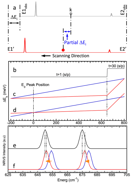
Figure 1. (a) A diagram to show the point-to-point energy correction procedure: k is the point index while i is the scan index; (b) the scanning time per data point (s/p) used in a conceptual NRVS between -200 cm-1 and +800 cm-1; (c) the energy correction at each data point assuming a total 0.8 meV energy drift per scan: the energy correction calibrated with a universal scale (blue) vs. that calibrated according to the accumulated time scanned (red); (d) the results from (c) with their zero energy peak position being aligned (to 0 cm-1); (e) a conceptual “raw” NRVS spectral section between 625 and 705 cm-1; (f) the NRVS spectra of (e) but calibrated with the two calibration methods used in (c) and (d) (color match).
In addition to the analysis with formulas, the two calibration processes can also be understood figuratively as the following. The region of 650 – 800 cm-1 accounts for (150/1000) = 15% of the whole energy range (from -200 cm-1 to 800 cm-1) but takes 30×150/(30×150+1×850) = 84% of the total scanning time. Therefore, an energy-scaled traditional calibration procedure [equation (1)] leads to 15% of the -0.8 meV (or -6.45 cm-1) energy drift being assigned to this region while a time-scaled calculation procedure [equation (4)] leads to 84% of the -0.8 meV being assigned to the same region, leaving -0.55 meV difference between the two calibration methods at 650 cm-1, as shown in Figure 1c. However, this -0.55 meV is not the real difference between the two calibration methods. After the zero energies for the two calibrations being re-aligned to 0 cm-1 as shown in Figure 1d, the maximum difference at 650 cm-1 becomes about -0.46 meV (Eerr1 = 0.46 meV) - this is the real energy difference between the two calibration methods. Assuming ΔEi=0.8 meV and ΔEcal=0.3 meV where ΔEcal stands for the energy drift amount when the calibration is performed, the errorbar due to the energy difference between different scans is estimated as Eerr2 = (ΔEi - ΔEcal) = 0.8 - 0.3 = 0.5 meV. In comparison, the Eerr1 (0.46 meV) is almost the same as Eerr2 (0.5 meV). In case that a ΔEi = 0.6 meV is assumed, Eerr1 = 0.35 meV while Eerr2 = 0.6 - 0.3 = 0.3 meV → Eerr1 > Eerr2. Therefore, Eerr1 is a critical portion of the total temperature drift-induced energy instabilities.
When an even scan is performed, the result from the equation (4) is the same as that from equation (5) [6][7]:
E’ = Eobs – {(E2obs–Eobs)/(E2obs–E1obs)}·ΔEi
= Eobs·{1+ΔEi/(E2obs–E1obs)}–{E2obs·ΔEi/(E2obs–E1obs)} (5)
Under this condition, it is reasonable to uniformly scale the Eobs according to the equation (5) [using αvar = {1+ΔEi/(E2obs–E1obs)}] rather than has to transform it point by point with equation (4). This establishes the concept that it is the nature of a sectional scan that makes it necessary to calibrate the observed energies point to point according to the accumulated beam-on time (Σtk), which is equation (4).
3. Re-Calibrating Published NRVS
How can researchers "re-calibrate" the published NRVS to add the time-scaled point to point re-distribution using equation (4)?
The first task is to reverse the original calibration process using the original α: E*obs = E*real/α, where E*real stands for the energy that was already calibrated with the traditional calibration procedure (1) while E*obs is a pseudo-observed energy back-converted (or it can be understood as the scan average of the original observed Eobs);
The second step is to convert the pseudo-observed data in E*obs to that in a new intermediate energy scale E’ using equation (4). For processing individual scans, ΔEi is used; for processing an averaged NRVS, a uniform ΔE can be used and obtained from averaging the ΔEi.
The last step is to use Ereal = E’·α0. The constant α0 is in principle a beamline-fixed constant and has to be obtained via a large amount of energy calibration data for each beamline [6][7]. The values can also be estimated by using equations (5) and (1):
α0 = α/{1+ΔE/(E2*obs–E1*obs)}
Ereal = E’·α0 (6)
This shows that α0 can be estimated from α, ΔE and (E2obs–E1obs).
With this procedure (6), small shifts of about -3 cm-1 is obtained for the X–Fe–H peaks for Chlamydomonas reinhardtii [FeFe] hydrogenase (or Cr HydA1 in short) [7]. Although the shift is not great, it is large enough to affect the comparison of some really small energy shifts, such as the 2 cm-1 between the CH-ADT and its C13D substituted counterpart in the same hydrogenase enzyme [7][11]. Researchers also noticed that the peak at 675 cm-1 has a bit more energy correction between the original and the re-calibrated spectra than the peak at 750 cm-1 does, which is consistent with the analysis in Figure 1c and 1d because the 30 s/p → 1 s/p scanning time changes at 650 cm-1 where is closer to 675 cm-1 than to ~750 cm-1. For details of this or other NRVS re-calibrations, please see the original reference [7].
4. Concluding Remarks
Based on the above discussion as well as the details in the recent publication [7], the following “conclusions” hold:
1) Due to the fact that the temperature induced energy drift is a function of time, the energy calibration (Eobs → Ereal) for a sectional scan should include a point by point re-distribution of the energy drift in each scan according to the time scanned [as in equations (4)] rather than be scaled with a universal constant [as in equation (1)];
2) The errorbar contributed from the improper “distribution” of ΔEi within each scan (Eerr1) is equally or sometimes more important than that due to the different ΔEi from scan to scan (Eerr2). Even without tracking the energy variation from scan to scan ΔEi but just re-distributing an averaged ΔE according to equation (4) or (6) can fix the Eerr1 and therefore reduce the total errorbar by ~50% [7];
3) The transition from the old calibration procedure (1) to the new calibration practice (4) takes time and some users may prefer to continue using the old calibration procedure (1). Under this circumstance, using multiple sections and less dramatic transition in scanning time makes its energy distribution curve closer to the one from an even energy calibration and thus leads to a smaller errorbar when equation (1) is used to to calibrate the energy axis;
4) No matter which calibration procedure is to be used and no matter what the scanning parameters are, no point should have an energy correction greater than the total energy drift per scan (ΔEi). Therefore, the final factor for controlling the possible energy calibration errors is to reduce ΔEi. For example, a) NRVS experiments need to wait for the beam energy to be stabilized (with less ΔEi per scan); b) the experimentalists also have the option to use less measurement time for each scan and take more scans to average instead.
This entry is adapted from the peer-reviewed paper 10.3390/physchem2040027
References
- Wang, H., et al., Nuclear Resonance Vibrational Spectroscopy: A Modern Tool to Pinpoint Site-Specific Cooperative Processes. Crystals, 2021. 11(8): p. 909.
- Wang, H., et al., Energy calibration issues in nuclear resonant vibrational spectroscopy: observing small spectral shifts and making fast calibrations. Journal of Synchrotron Radiation, 2013. 20(5): p. 683-690.
- Wang, H., et al., A Practical Guide for Nuclear Resonance Vibrational Spectroscopy (NRVS) of Biochemical Samples and Model Compounds, in Metalloproteins, J.C. Fontecilla-Camps and Y. Nicolet, Editors. 2014, Humana Press. p. 125-137.
- Wang, J., L. Li, and H. Wang, Machine learning concept in de-spiking process for nuclear resonant vibrational spectra – Automation using no external parameter. Vibrational Spectroscopy, 2022. 119: p. 103352.
- Wang, H., et al., L-edge sum rule analysis on 3d transition metal sites: from d10 to d0 and towards application to extremely dilute metallo-enzymes. Physical Chemistry Chemical Physics, 2018. 20(12): p. 8166-8176.
- Wang, J., Y. Yoda, and H. Wang, Tracking energy scale variations from scan to scan in nuclear resonant vibrational spectroscopy: In situ correction using zero-energy position drifts ΔEi rather than making in situ calibration measurements. Review of Scientific Instruments, 2022. 93(9): p. 095101.
- Wang, H., Y. Yoda, and J. Wang, The True Nature of the Energy Calibration for Nuclear Resonant Vibrational Spectroscopy: A Time-Based Conversion. Physchem, 2022. 2(4): p. 369-389.
- Wang, H., et al., A strenuous experimental journey searching for spectroscopic evidence of a bridging nickel-iron-hydride in [NiFe] hydrogenase. Journal of Synchrotron Radiation, 2015. 22(6): p. 1334-1344.
- Ogata, H., et al., Hydride bridge in [NiFe]-hydrogenase observed by nuclear resonance vibrational spectroscopy. Nat Commun, 2015. 6: p. 7890.
- Pham, C.C., et al., Terminal Hydride Species in [FeFe]-Hydrogenases are Vibrationally Coupled to the Active Site Environment. Angewandte Chemie-International Edition, 2018. 57(33): p. 10605-10609.
- Pelmenschikov, V., et al., Vibrational Perturbation of the [FeFe] Hydrogenase H-Cluster Revealed by 13C2H-ADT Labeling. Journal of the American Chemical Society, 2021.
- Lumen-Physics. Heat and Heat Transfer Methods. 2016; Available from: https://courses.lumenlearning.com/physics/chapter/14-5-conduction/.