1. Definition

Formally, reduce takes an associative (but not necessarily commutative) operator [math]\displaystyle{ \oplus }[/math], which can be evaluated in constant time and an input set [math]\displaystyle{ V = \{v_0 = \begin{pmatrix} e_0^0 \\ \vdots \\ e_0^{m-1}\end{pmatrix}, v_1 = \begin{pmatrix} e_1^0 \\ \vdots \\ e_1^{m-1}\end{pmatrix}, \dots, v_{p-1} = \begin{pmatrix} e_{p-1}^0 \\ \vdots \\ e_{p-1}^{m-1}\end{pmatrix}\} }[/math]of [math]\displaystyle{ p }[/math] vectors with [math]\displaystyle{ m }[/math] elements each. The total size of a vector is defined as [math]\displaystyle{ n }[/math]. The result [math]\displaystyle{ r }[/math] of the operation is the combination of the elements [math]\displaystyle{ r = \begin{pmatrix} e_0^0 \oplus e_1^0 \oplus \dots \oplus e_{p-1}^0 \\ \vdots \\ e_0^{m-1} \oplus e_1^{m-1} \oplus \dots \oplus e_{p-1}^{m-1}\end{pmatrix} = \begin{pmatrix} \bigoplus_{i=0}^{p-1} e_i^0 \\ \vdots \\ \bigoplus_{i=0}^{p-1} e_i^{m-1} \end{pmatrix} }[/math] and has to be stored at a specified root processor at the end of the execution. For example, the result of a reduction on the set [math]\displaystyle{ \{3,5,7,9\} }[/math], where all vectors have size one is [math]\displaystyle{ 3 + 5 + 7 + 9 = 24 }[/math]. If the result [math]\displaystyle{ r }[/math] has to be available at every processor after the computation has finished, it is often called Allreduce. An optimal sequential linear-time algorithm for reduction can apply the operator successively from front to back, always replacing two vectors with the result of the operation applied to all its elements, thus creating an instance that has one vector less. It needs [math]\displaystyle{ (p-1)\cdot m }[/math] steps until only [math]\displaystyle{ r }[/math] is left. Sequential algorithms can not perform better than linear time, but parallel algorithms leave some space left to optimize.

2. Binomial Tree Algorithms

Regarding parallel algorithms, there are two main models of parallel computation, the parallel random access machine as an extension of the RAM with shared memory between processing units and the bulk synchronous parallel computer which takes communication and synchronization into account. Both models have different implications for the time-complexity, therefore two algorithms will be shown.

2.1. PRAM-Algorithm

This algorithm represents a widely spread method to handle inputs where [math]\displaystyle{ p }[/math] is a power of two. The reverse procedure is often used for broadcasting elements.^[1][2][3]

Visualization of the algorithm executed on eight elements using addition as the operator. https://handwiki.org/wiki/index.php?curid=1214953

for [math]\displaystyle{ k \gets 0 }[/math] to [math]\displaystyle{ \lceil\log_2 p\rceil - 1 }[/math] do

for [math]\displaystyle{ i \gets 0 }[/math] to [math]\displaystyle{ p - 1 }[/math] do in parallel

if [math]\displaystyle{ p_i }[/math] is active then

if bit [math]\displaystyle{ k }[/math] of [math]\displaystyle{ i }[/math] is set then

set [math]\displaystyle{ p_i }[/math] to inactive

else if [math]\displaystyle{ i + 2^k \lt p }[/math]

[math]\displaystyle{ x_i \gets x_i \oplus^{\star} x_{i+2^k} }[/math]

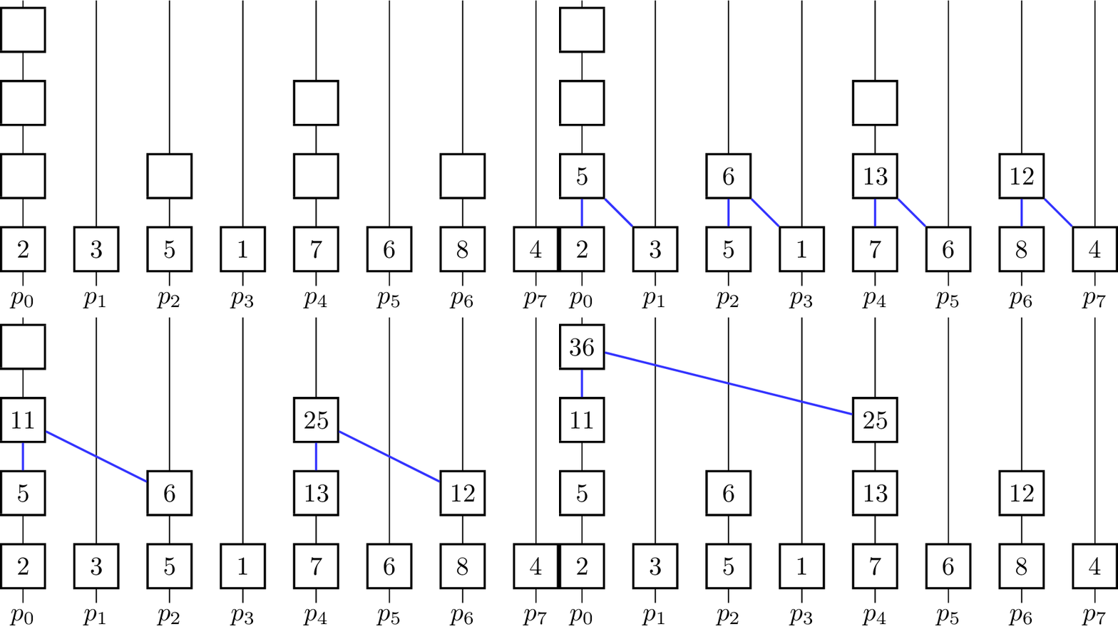
The binary operator for vectors is defined such that [math]\displaystyle{ \begin{pmatrix} e_i^0 \\ \vdots \\ e_i^{m-1}\end{pmatrix} \oplus^\star \begin{pmatrix} e_j^0 \\ \vdots \\ e_j^{m-1}\end{pmatrix} = \begin{pmatrix} e_i^0 \oplus e_j^0 \\ \vdots \\ e_i^{m-1} \oplus e_j^{m-1} \end{pmatrix} }[/math]. The algorithm further assumes that in the beginning [math]\displaystyle{ x_i = v_i }[/math] for all [math]\displaystyle{ i }[/math] and [math]\displaystyle{ p }[/math] is a power of two and uses the processing units [math]\displaystyle{ p_0, p_1,\dots p_{n-1} }[/math]. In every iteration, half of the processing units become inactive and do not contribute to further computations. The figure shows a visualization of the algorithm using addition as the operator. Vertical lines represent the processing units where the computation of the elements on that line take place. The eight input elements are located on the bottom and every animation step corresponds to one parallel step in the execution of the algorithm. An active processor [math]\displaystyle{ p_i }[/math] evaluates the given operator on the element [math]\displaystyle{ x_i }[/math] it is currently holding and [math]\displaystyle{ x_j }[/math] where [math]\displaystyle{ j }[/math] is the minimal index fulfilling [math]\displaystyle{ j \gt i }[/math], so that [math]\displaystyle{ p_j }[/math] is becoming an inactive processor in the current step. [math]\displaystyle{ x_i }[/math] and [math]\displaystyle{ x_j }[/math] are not necessarily elements of the input set [math]\displaystyle{ X }[/math] as the fields are overwritten and reused for previously evaluated expressions. To coordinate the roles of the processing units in each step without causing additional communication between them, the fact that the processing units are indexed with numbers from [math]\displaystyle{ 0 }[/math] to [math]\displaystyle{ p-1 }[/math] is used. Each processor looks at its [math]\displaystyle{ k }[/math]-th least significant bit and decides whether to get inactive or compute the operator on its own element and the element with the index where the [math]\displaystyle{ k }[/math]-th bit is not set. The underlying communication pattern of the algorithm is a binomial tree, hence the name of the algorithm.

Only [math]\displaystyle{ p_0 }[/math] holds the result in the end, therefore it is the root processor. For an Allreduce-operation the result has to be distributed, which can be done by appending a broadcast from [math]\displaystyle{ p_0 }[/math]. Furthermore, the number [math]\displaystyle{ p }[/math] of processors is restricted to be a power of two. This can be lifted by padding the number of processors to the next power of two. There are also algorithms that are more tailored for this use-case.^[4]

Runtime analysis

The main loop is executed [math]\displaystyle{ \lceil\log_2 p\rceil }[/math] times, the time needed for the part done in parallel is in [math]\displaystyle{ \mathcal{O}(m) }[/math] as a processing unit either combines two vectors or becomes inactive. Thus the parallel time [math]\displaystyle{ T(p, m) }[/math] for the PRAM is [math]\displaystyle{ T(p, m) = \mathcal{O}(\log(p) \cdot m) }[/math]. The strategy for handling read and write conflicts can be chosen as restrictive as an exclusive read and exclusive write (EREW). The efficiency [math]\displaystyle{ S(p, m) }[/math] of the algorithm is [math]\displaystyle{ S(p, m) \in \mathcal{O}(\frac{T_{seq}}{T(p, m)}) = \mathcal{O}(\frac{p}{\log(p)}) }[/math] and therefore the efficiency is [math]\displaystyle{ E(p, m) \in \mathcal{O}(\frac{S(p, m)}{p}) = \mathcal{O}(\frac{1}{\log(p)}) }[/math]. The efficiency suffers because of the fact that half of the active processing units become inactive after each step, so [math]\displaystyle{ \frac{p}{2^i} }[/math] units are active in step [math]\displaystyle{ i }[/math].

2.2. Distributed Memory Algorithm

In contrast to the PRAM-algorithm, in the distributed memory model memory is not shared between processing units and data has to be exchanged explicitly between units, resulting in communication overhead that is accounted for. The following algorithm takes this into consideration.

for [math]\displaystyle{ k \gets 0 }[/math] to [math]\displaystyle{ \lceil\log_2 p\rceil - 1 }[/math] do

for [math]\displaystyle{ i \gets 0 }[/math] to [math]\displaystyle{ p - 1 }[/math] do in parallel

if [math]\displaystyle{ p_i }[/math] is active then

if bit [math]\displaystyle{ k }[/math] of [math]\displaystyle{ i }[/math] is set then

send [math]\displaystyle{ x_i }[/math] to [math]\displaystyle{ p_{i-2^k} }[/math]

set [math]\displaystyle{ p_k }[/math] to inactive

else if [math]\displaystyle{ i + 2^k \lt p }[/math]

receive [math]\displaystyle{ x_{i+2^k} }[/math]

[math]\displaystyle{ x_i \gets x_i \oplus^\star x_{i+2^k} }[/math]

The only difference between the distributed algorithm and the PRAM version is the inclusion of explicit communication primitives, the operating principle stays the same.

Runtime analysis

A simple analysis for the algorithm uses the BSP-model and incorporates the time [math]\displaystyle{ T_{start} }[/math] needed to initiate communication and [math]\displaystyle{ T_{byte} }[/math] the time needed to send a byte. Then the resulting runtime is [math]\displaystyle{ \Theta((T_{start} + n \cdot T_{byte})\cdot log(p)) }[/math], as [math]\displaystyle{ m }[/math] elements of a vector are sent in each iteration and have size [math]\displaystyle{ n }[/math] in total.

3. Pipeline-Algorithm

Depiction of the pipeline-algorithm using addition as the operator on vectors of size four. https://handwiki.org/wiki/index.php?curid=1093982

For distributed memory models, it can make sense to use pipelined communication. This is especially the case when [math]\displaystyle{ T_{start} }[/math] is small in comparison to [math]\displaystyle{ T_{byte} }[/math]. Usually, linear pipelines split data or a task into smaller pieces and process them in stages. In contrast to the binomial tree algorithms, the pipelined algorithm uses the fact that the vectors are not inseparable, but the operator can be evaluated for single elements:^[5]

for [math]\displaystyle{ k \gets 0 }[/math] to [math]\displaystyle{ p+m-3 }[/math] do

for [math]\displaystyle{ i \gets 0 }[/math] to [math]\displaystyle{ p - 1 }[/math] do in parallel

if [math]\displaystyle{ i \leq k \lt i+m \land i \neq p-1 }[/math]

send [math]\displaystyle{ x_i^{k-i} }[/math] to [math]\displaystyle{ p_{i+1} }[/math]

if [math]\displaystyle{ i-1 \leq k \lt i-1+m \land i \neq 0 }[/math]

receive [math]\displaystyle{ x_{i-1}^{k+i-1} }[/math] from [math]\displaystyle{ p_{i-1} }[/math]

[math]\displaystyle{ x_{i}^{k+i-1} \gets x_{i}^{k+i-1} \oplus x_{i-1}^{k+i-1} }[/math]

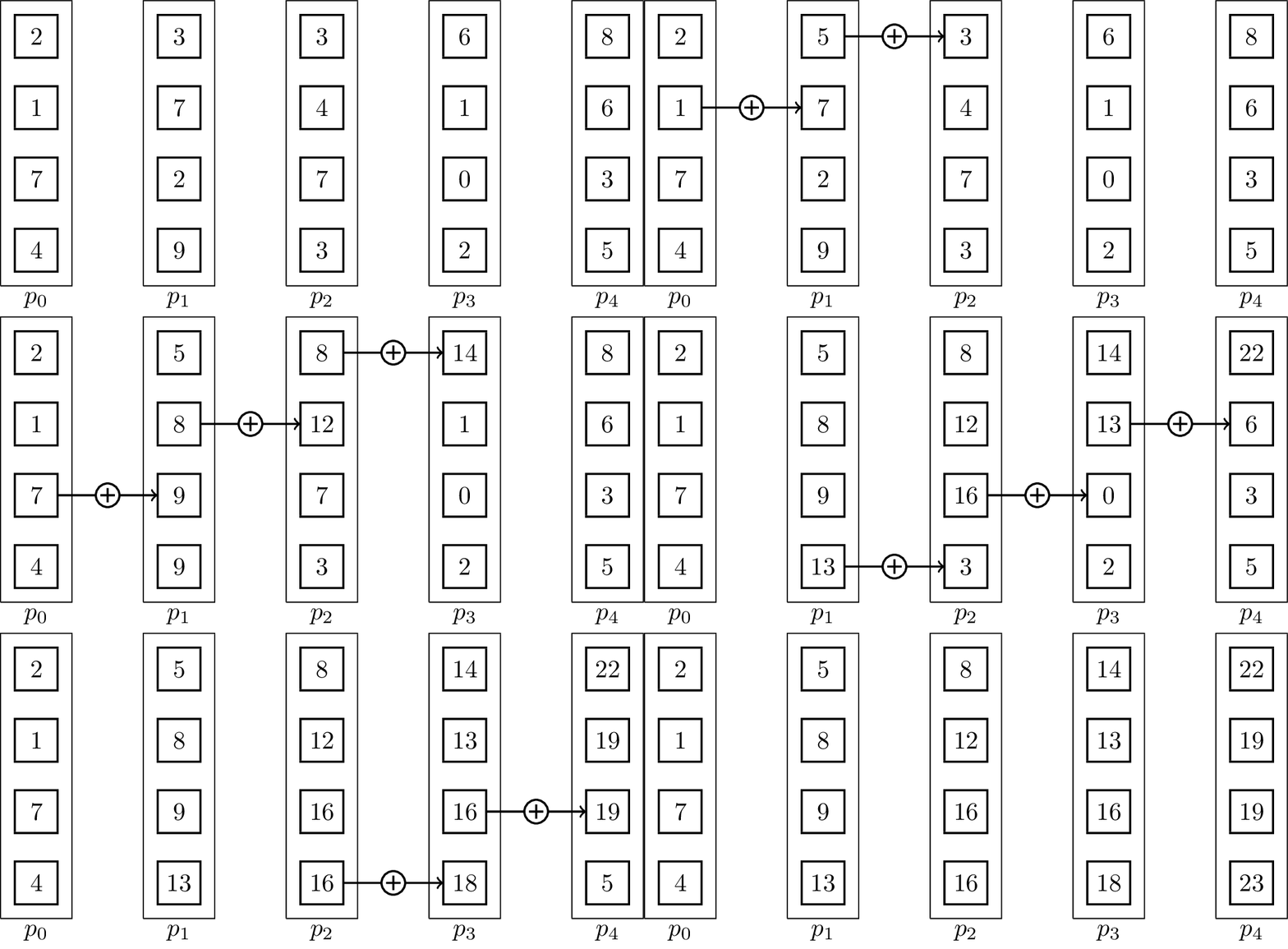
It is important to note that the send and receive operations have to be executed concurrently for the algorithm to work. The result vector is stored at [math]\displaystyle{ p_{p-1} }[/math] at the end. The associated animation shows an execution of the algorithm on vectors of size four with five processing units. Two steps of the animation visualize one parallel execution step. The number of steps in the parallel execution are [math]\displaystyle{ p + m -2 }[/math], it takes [math]\displaystyle{ p-1 }[/math] steps until the last processing unit receives its first element and additional [math]\displaystyle{ m-1 }[/math] until all elements are received. Therefore, the runtime in the BSP-model is [math]\displaystyle{ T(n, p, m) = (T_{start} + \frac{n}{m}T_{byte})(p+m-2) }[/math], assuming that [math]\displaystyle{ n }[/math] is the total byte-size of a vector.

Although [math]\displaystyle{ m }[/math] has a fixed value, it is possible to logically group elements of a vector together and reduce [math]\displaystyle{ m }[/math]. For example, a problem instance with vectors of size four can be handled by splitting the vectors into the first two and last two elements, which are always transmitted and computed together. In this case, double the volume is sent each step, but the number of steps has roughly halved. It means that the parameter [math]\displaystyle{ m }[/math] is halved, while the total byte-size [math]\displaystyle{ n }[/math] stays the same. The runtime [math]\displaystyle{ T(p) }[/math] for this approach depends on the value of [math]\displaystyle{ m }[/math], which can be optimized if [math]\displaystyle{ T_{start} }[/math] and [math]\displaystyle{ T_{byte} }[/math] are known. It is optimal for [math]\displaystyle{ m = \sqrt{\frac{n \cdot (p-2)T_{byte}}{T_{start}}} }[/math], assuming that this results in a smaller [math]\displaystyle{ m }[/math] that divides the original one.

4. Pipelined Tree

Pipelined Fibonacci-tree algorithm using addition. https://handwiki.org/wiki/index.php?curid=1981174

The binomial tree and the pipeline both have their advantages and disadvantages, depending on the values of [math]\displaystyle{ T_{start} }[/math] and [math]\displaystyle{ T_{byte} }[/math] for the parallel communication. While the binomial tree algorithm is better suited for small vectors, the pipelined algorithm profits from a distribution of the elements to fewer processing units with more elements contained in one vector. Both approaches can be combined into one algorithm^[6] which uses a tree as its underlying communication pattern and splits the computation of the operator into pieces at the same time. Instead of the binomial tree, a Fibonacci tree is used which has the property that the height of the trees rooted at its two children differ by one. It helps to balance the load on all processing units as each unit can only evaluate one operator in one iteration on one of its elements, but it has two child-processors it receives values from.

4.1. Algorithm Description

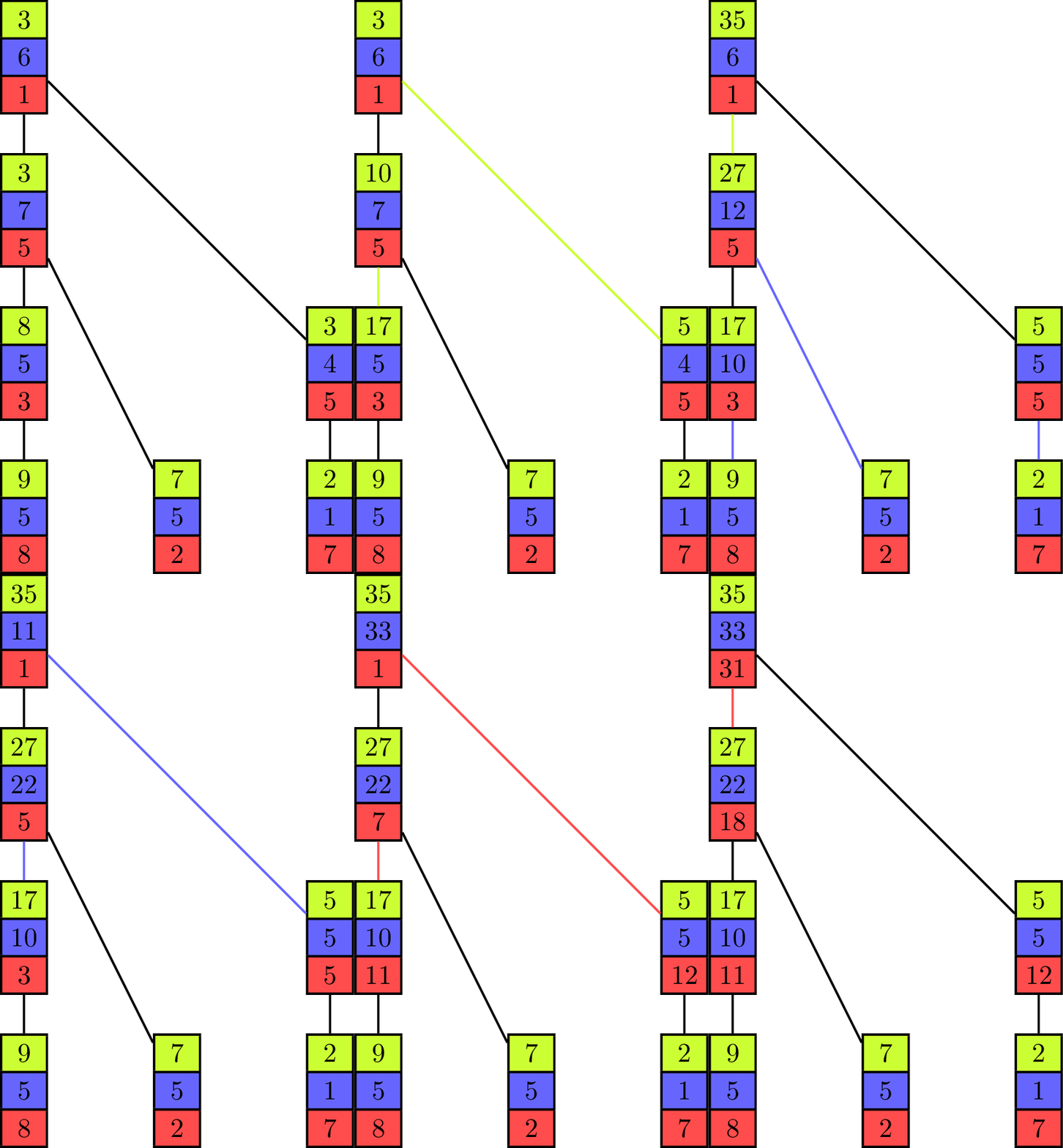
The animation shows the execution of such an algorithm in a full-duplex communication model. Communication links are represented by black lines between the vectors of elements and build a Fibonacci tree of size seven in this example. If an element is sent to another processing unit the link is colored with the color of the corresponding element. An element that is received by a processor is added to the already existing element of same color (at the same index in the vector).

The algorithm itself propagates the partial sums from bottom to top until all elements are contained in the sum at the root processor on top. In the first step of the execution, the processing units which are leaves in the underlying tree send their first elements to their parent. This is similar to the send operations of the binomial tree algorithm with the key difference that the leaf units each have two more elements which have to be sent and therefore do not become inactive, but can continue to send elements, which is analogous to the pipelined approach and improves efficiency. Processing units that are not leaves start to send their elements in order of the indices in the vector once they have received an element from a child. In the example they send green, blue and red elements in this order. If two processors compete to send their elements to the same processor, then the element of the right child is received first. Because of the structure of the Fibonacci tree all processors send or receive elements while the "pipeline" is filled. The pipeline is filled from the point where each unit has received an element and until the leaf units have no more elements to send.

4.2. Runtime

Each iteration of the algorithm takes at most time [math]\displaystyle{ \frac{n}{m} \cdot T_{byte} + T_{start} }[/math]. The height of the tree factors into the time it needs to fill the pipeline and for Fibonacci trees it is known to be about [math]\displaystyle{ h = log_{\phi}p }[/math] where [math]\displaystyle{ \phi = \frac{1 + \sqrt{5}}{2} }[/math] is the golden ratio. Once the pipeline is filled, all processors are active in each step. Because inner nodes have two children, they have to receive [math]\displaystyle{ 2 \cdot m }[/math] elements. Therefore, the runtime of the algorithm is [math]\displaystyle{ T(n, p, m) \approx (\frac{n}{m} \cdot T_{byte} + T_{start})(h + 2 \cdot k - 2) }[/math]. It is minimal if the number of elements in a vector is chosen such that [math]\displaystyle{ m = \sqrt{\frac{n \cdot (h-3)T_{byte}}{3 \cdot T_{start}}} }[/math].

5. Applications

Reduction is one of the main collective operations implemented in the Message Passing Interface, where performance of the used algorithm is important and evaluated constantly for different use cases.^[7]

MapReduce relies heavily on efficient reduction algorithms to process big data sets, even on huge clusters.^[8][9]

Some parallel sorting algorithms use reductions to be able to handle very big data sets.^[10]

The content is sourced from: https://handwiki.org/wiki/Reduce_(parallel_pattern)

References

- Bar-Noy, Amotz; Kipnis, Shlomo (1994). "Broadcasting multiple messages in simultaneous send/receive systems". Discrete Applied Mathematics 55 (2): 95–105. doi:10.1016/0166-218x(94)90001-9. https://dx.doi.org/10.1016%2F0166-218x%2894%2990001-9
- Santos, Eunice E. (2002). "Optimal and Efficient Algorithms for Summing and Prefix Summing on Parallel Machines". Journal of Parallel and Distributed Computing 62 (4): 517–543. doi:10.1006/jpdc.2000.1698. https://dx.doi.org/10.1006%2Fjpdc.2000.1698
- Slater, P.; Cockayne, E.; Hedetniemi, S. (1981-11-01). "Information Dissemination in Trees". SIAM Journal on Computing 10 (4): 692–701. doi:10.1137/0210052. ISSN 0097-5397. https://dx.doi.org/10.1137%2F0210052
- Rabenseifner, Rolf; Träff, Jesper Larsson (2004-09-19) (in en). More Efficient Reduction Algorithms for Non-Power-of-Two Number of Processors in Message-Passing Parallel Systems. Lecture Notes in Computer Science. 3241. Springer, Berlin, Heidelberg. 36–46. doi:10.1007/978-3-540-30218-6_13. ISBN 9783540231639. https://dx.doi.org/10.1007%2F978-3-540-30218-6_13
- Bar-Noy, A.; Kipnis, S. (1994-09-01). "Designing broadcasting algorithms in the postal model for message-passing systems" (in en). Mathematical Systems Theory 27 (5): 431–452. doi:10.1007/BF01184933. ISSN 0025-5661. https://dx.doi.org/10.1007%2FBF01184933
- Sanders, Peter; Sibeyn, Jop F (2003). "A bandwidth latency tradeoff for broadcast and reduction". Information Processing Letters 86 (1): 33–38. doi:10.1016/s0020-0190(02)00473-8. https://dx.doi.org/10.1016%2Fs0020-0190%2802%2900473-8
- Pješivac-Grbović, Jelena; Angskun, Thara; Bosilca, George; Fagg, Graham E.; Gabriel, Edgar; Dongarra, Jack J. (2007-06-01). "Performance analysis of MPI collective operations" (in en). Cluster Computing 10 (2): 127–143. doi:10.1007/s10586-007-0012-0. ISSN 1386-7857. https://dx.doi.org/10.1007%2Fs10586-007-0012-0
- Lämmel, Ralf (2008). "Google's MapReduce programming model — Revisited". Science of Computer Programming 70 (1): 1–30. doi:10.1016/j.scico.2007.07.001. https://dx.doi.org/10.1016%2Fj.scico.2007.07.001
- Senger, Hermes; Gil-Costa, Veronica; Arantes, Luciana; Marcondes, Cesar A. C.; Marín, Mauricio; Sato, Liria M.; da Silva, Fabrício A.B. (2016-06-10). "BSP cost and scalability analysis for MapReduce operations" (in en). Concurrency and Computation: Practice and Experience 28 (8): 2503–2527. doi:10.1002/cpe.3628. ISSN 1532-0634. https://dx.doi.org/10.1002%2Fcpe.3628
- Axtmann, Michael; Bingmann, Timo; Sanders, Peter; Schulz, Christian (2014-10-24). "Practical Massively Parallel Sorting". arXiv:1410.6754 [cs.DS]. //arxiv.org/archive/cs.DS