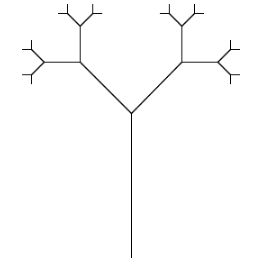
-

Axiom. https://handwiki.org/wiki/index.php?curid=1266298
-

First recursion. https://handwiki.org/wiki/index.php?curid=1575494
-
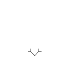
Second recursion. https://handwiki.org/wiki/index.php?curid=1930274
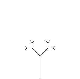
-
Third recursion. https://handwiki.org/wiki/index.php?curid=1488101
-
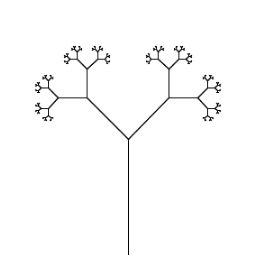
Seventh recursion, scaled down ten times. https://handwiki.org/wiki/index.php?curid=1595774
An L-system or Lindenmayer system is a parallel rewriting system and a type of formal grammar. An L-system consists of an alphabet of symbols that can be used to make strings, a collection of production rules that expand each symbol into some larger string of symbols, an initial "axiom" string from which to begin construction, and a mechanism for translating the generated strings into geometric structures. L-systems were introduced and developed in 1968 by Aristid Lindenmayer, a Hungarian theoretical biologist and botanist at the University of Utrecht. Lindenmayer used L-systems to describe the behaviour of plant cells and to model the growth processes of plant development. L-systems have also been used to model the morphology of a variety of organisms and can be used to generate self-similar fractals.
- plant cells
- fractals
- model
1. Origins
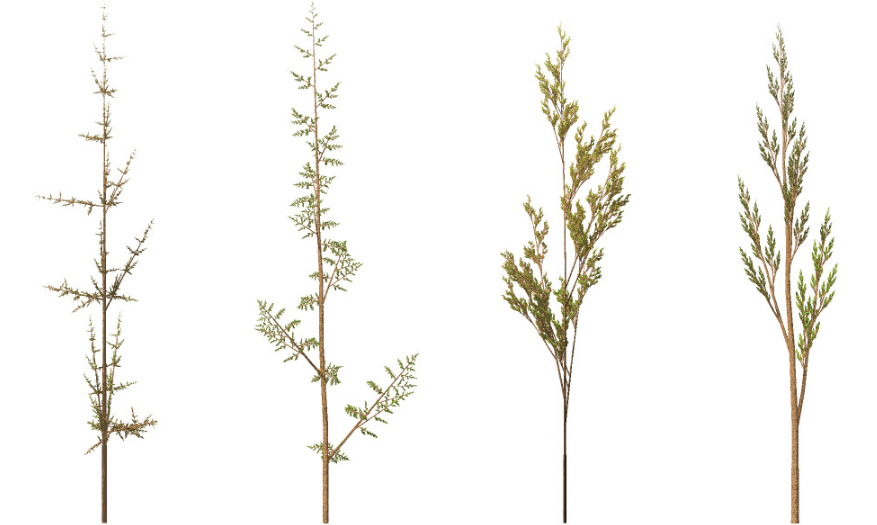
As a biologist, Lindenmayer worked with yeast and filamentous fungi and studied the growth patterns of various types of bacteria, such as the cyanobacteria Anabaena catenula. Originally the L-systems were devised to provide a formal description of the development of such simple multicellular organisms, and to illustrate the neighbourhood relationships between plant cells. Later on, this system was extended to describe higher plants and complex branching structures.
2. L-system Structure
The recursive nature of the L-system rules leads to self-similarity and thereby, fractal-like forms are easy to describe with an L-system. Plant models and natural-looking organic forms are easy to define, as by increasing the recursion level the form slowly 'grows' and becomes more complex. Lindenmayer systems are also popular in the generation of artificial life.
L-system grammars are very similar to the semi-Thue grammar (see Chomsky hierarchy). L-systems are now commonly known as parametric L systems, defined as a tuple
- G = (V, ω, P),
where
- V (the alphabet) is a set of symbols containing both elements that can be replaced (variables) and those which cannot be replaced ("constants" or "terminals")
- ω (start, axiom or initiator) is a string of symbols from V defining the initial state of the system
- P is a set of production rules or productions defining the way variables can be replaced with combinations of constants and other variables. A production consists of two strings, the predecessor and the successor. For any symbol A which is a member of the set V which does not appear on the left hand side of a production in P, the identity production A → A is assumed; these symbols are called constants or terminals. (See Law of identity).
The rules of the L-system grammar are applied iteratively starting from the initial state. As many rules as possible are applied simultaneously, per iteration. The fact that each iteration employs as many rules as possible differentiates an L-system from a formal language generated by a formal grammar, which applies only one rule per iteration. If the production rules were to be applied only one at a time, one would quite simply generate a language, rather than an L-system.[clarification needed]Thus, L-systems are strict subsets of languages.[clarification needed]
An L-system is context-free if each production rule refers only to an individual symbol and not to its neighbours. Context-free L-systems are thus specified by a context-free grammar. If a rule depends not only on a single symbol but also on its neighbours, it is termed a context-sensitive L-system.
If there is exactly one production for each symbol, then the L-system is said to be deterministic (a deterministic context-free L-system is popularly called a D0L system). If there are several, and each is chosen with a certain probability during each iteration, then it is a stochastic L-system.
Using L-systems for generating graphical images requires that the symbols in the model refer to elements of a drawing on the computer screen. For example, the program Fractint uses turtle graphics (similar to those in the Logo programming language) to produce screen images. It interprets each constant in an L-system model as a turtle command.
3. Examples of L-systems
3.1. Example 1: Algae
Lindenmayer's original L-system for modelling the growth of algae.
- variables : A B
- constants : none
- axiom : A
- rules : (A → AB), (B → A)
which produces:
- n = 0 : A
- n = 1 : AB
- n = 2 : ABA
- n = 3 : ABAAB
- n = 4 : ABAABABA
- n = 5 : ABAABABAABAAB
- n = 6 : ABAABABAABAABABAABABA
- n = 7 : ABAABABAABAABABAABABAABAABABAABAAB
3.2. Example 1: Algae, Explained
n=0: A start (axiom/initiator) / \ n=1: A B the initial single A spawned into AB by rule (A → AB), rule (B → A) couldn't be applied /| \ n=2: A B A former string AB with all rules applied, A spawned into AB again, former B turned into A /| | |\ n=3: A B A A B note all A's producing a copy of themselves in the first place, then a B, which turns ... /| | |\ |\ \ n=4: A B A A B A B A ... into an A one generation later, starting to spawn/repeat/recurse then
The result is the sequence of Fibonacci words. If we count the length of each string, we obtain the famous Fibonacci sequence of numbers (skipping the first 1, due to our choice of axiom):
- 1 2 3 5 8 13 21 34 55 89 ...
For each string, if we count the k-th position from the left end of the string, the value is determined by whether a multiple of the golden ratio falls within the interval [math]\displaystyle{ (k-1, k) }[/math]. The ratio of A to B likewise converges to the golden mean.
This example yields the same result (in terms of the length of each string, not the sequence of As and Bs) if the rule (A → AB) is replaced with (A → BA), except that the strings are mirrored.
This sequence is a locally catenative sequence because [math]\displaystyle{ G(n)=G(n-1)G(n-2) }[/math], where [math]\displaystyle{ G(n) }[/math] is the n-th generation.
3.2. Example 2: Fractal (Binary) Tree
- variables : 0, 1
- constants: [, ]
- axiom : 0
- rules : (1 → 11), (0 → 1[0]0)
The shape is built by recursively feeding the axiom through the production rules. Each character of the input string is checked against the rule list to determine which character or string to replace it with in the output string. In this example, a '1' in the input string becomes '11' in the output string, while '[' remains the same. Applying this to the axiom of '0', we get:
| axiom: | 0 |
| 1st recursion: | 1[0]0 |
| 2nd recursion: | 11[1[0]0]1[0]0 |
| 3rd recursion: | 1111[11[1[0]0]1[0]0]11[1[0]0]1[0]0 |
| … |
We can see that this string quickly grows in size and complexity. This string can be drawn as an image by using turtle graphics, where each symbol is assigned a graphical operation for the turtle to perform. For example, in the sample above, the turtle may be given the following instructions:
- 0: draw a line segment ending in a leaf
- 1: draw a line segment
- [: push position and angle, turn left 45 degrees
- ]: pop position and angle, turn right 45 degrees
The push and pop refer to a LIFO stack (more technical grammar would have separate symbols for "push position" and "turn left"). When the turtle interpretation encounters a '[', the current position and angle are saved, and are then restored when the interpretation encounters a ']'. If multiple values have been "pushed," then a "pop" restores the most recently saved values. Applying the graphical rules listed above to the earlier recursion, we get:
3.3. Example 3: Cantor Set

- variables : A B
- constants : none
- start : A {starting character string}
- rules : (A → ABA), (B → BBB)
Let A mean "draw forward" and B mean "move forward".
This produces the famous Cantor's fractal set on a real straight line R.
3.4. Example 4: Koch Curve
A variant of the Koch curve which uses only right angles.
- variables : F
- constants : + −
- start : F
- rules : (F → F+F−F−F+F)
Here, F means "draw forward", + means "turn left 90°", and − means "turn right 90°" (see turtle graphics).
- n = 0:
- F
- n = 1:
- F+F−F−F+F
- n = 2:
- F+F−F−F+F + F+F−F−F+F − F+F−F−F+F − F+F−F−F+F + F+F−F−F+F
- n = 3:
- F+F−F−F+F+F+F−F−F+F−F+F−F−F+F−F+F−F−F+F+F+F−F−F+F +
- F+F−F−F+F+F+F−F−F+F−F+F−F−F+F−F+F−F−F+F+F+F−F−F+F −
- F+F−F−F+F+F+F−F−F+F−F+F−F−F+F−F+F−F−F+F+F+F−F−F+F −
- F+F−F−F+F+F+F−F−F+F−F+F−F−F+F−F+F−F−F+F+F+F−F−F+F +
- F+F−F−F+F+F+F−F−F+F−F+F−F−F+F−F+F−F−F+F+F+F−F−F+F
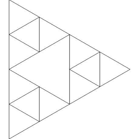
3.5. Example 5: Sierpinski Triangle
The Sierpinski triangle drawn using an L-system.
- variables : F G
- constants : + −
- start : F−G−G
- rules : (F → F−G+F+G−F), (G → GG)
- angle : 120°
Here, F and G both mean "draw forward", + means "turn left by angle", and − means "turn right by angle".
-
-
n = 2. https://handwiki.org/wiki/index.php?curid=1686333
-
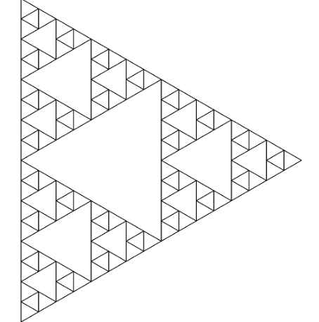
n = 4. https://handwiki.org/wiki/index.php?curid=1087772
-
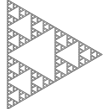
n = 6. https://handwiki.org/wiki/index.php?curid=1760444
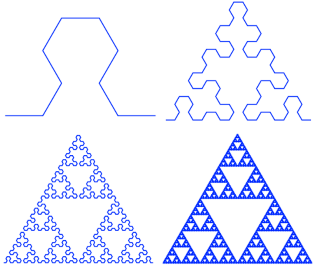
It is also possible to approximate the Sierpinski triangle using a Sierpiński arrowhead curve L-system.
- variables : A B
- constants : + −
- start : A
- rules : (A → B−A−B), (B → A+B+A)
- angle : 60°
Here, A and B both mean "draw forward", + means "turn left by angle", and − means "turn right by angle" (see turtle graphics).
3.6. Example 6: Dragon Curve
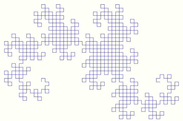
The dragon curve drawn using an L-system.
- variables : X Y
- constants : F + −
- start : FX
- rules : (X → X+YF+), (Y → −FX−Y)
- angle : 90°
Here, F means "draw forward", − means "turn left 90°", and + means "turn right 90°". X and Y do not correspond to any drawing action and are only used to control the evolution of the curve.
3.7. Example 7: Fractal Plant
- variables : X F
- constants : + − [ ]
- start : X
- rules : (X → F+[[X]-X]-F[-FX]+X), (F → FF)
- angle : 25°
Here, F means "draw forward", − means "turn left 25°", and + means "turn right 25°". X does not correspond to any drawing action and is used to control the evolution of the curve. The square bracket "[" corresponds to saving the current values for position and angle, which are restored when the corresponding "]" is executed.

4. Variations
A number of elaborations on this basic L-system technique have been developed which can be used in conjunction with each other. Among these are stochastic grammars, context sensitive grammars, and parametric grammars.
4.1. Stochastic Grammars
The grammar model we have discussed thus far has been deterministic—that is, given any symbol in the grammar's alphabet, there has been exactly one production rule, which is always chosen, and always performs the same conversion. One alternative is to specify more than one production rule for a symbol, giving each a probability of occurring. For example, in the grammar of Example 2, we could change the rule for rewriting "0" from:
- 0 → 1[0]0
to a probabilistic rule:
- 0 (0.5) → 1[0]0
- 0 (0.5) → 0
Under this production, whenever a "0" is encountered during string rewriting, there would be a 50% chance it would behave as previously described, and a 50% chance it would not change during production. When a stochastic grammar is used in an evolutionary context, it is advisable to incorporate a random seed into the genotype, so that the stochastic properties of the image remain constant between generations.
4.2. Context Sensitive Grammars
A context sensitive production rule looks not only at the symbol it is modifying, but the symbols on the string appearing before and after it. For instance, the production rule:
- b < a > c → aa
transforms "a" to "aa", but only If the "a" occurs between a "b" and a "c" in the input string:
- …bac…
As with stochastic productions, there are multiple productions to handle symbols in different contexts. If no production rule can be found for a given context, the identity production is assumed, and the symbol does not change on transformation. If context-sensitive and context-free productions both exist within the same grammar, the context-sensitive production is assumed to take precedence when it is applicable.
4.3. Parametric Grammars
In a parametric grammar, each symbol in the alphabet has a parameter list associated with it. A symbol coupled with its parameter list is called a module, and a string in a parametric grammar is a series of modules. An example string might be:
- a(0,1)[b(0,0)]a(1,2)
The parameters can be used by the drawing functions, and also by the production rules. The production rules can use the parameters in two ways: first, in a conditional statement determining whether the rule will apply, and second, the production rule can modify the actual parameters. For example, look at:
- a(x,y) : x == 0 → a(1, y+1)b(2,3)
The module a(x,y) undergoes transformation under this production rule if the conditional x=0 is met. For example, a(0,2) would undergo transformation, and a(1,2) would not.
In the transformation portion of the production rule, the parameters as well as entire modules can be affected. In the above example, the module b(x,y) is added to the string, with initial parameters (2,3). Also, the parameters of the already existing module are transformed. Under the above production rule,
- a(0,2)
Becomes
- a(1,3)b(2,3)
as the "x" parameter of a(x,y) is explicitly transformed to a "1" and the "y" parameter of a is incremented by one.
Parametric grammars allow line lengths and branching angles to be determined by the grammar, rather than the turtle interpretation methods. Also, if age is given as a parameter for a module, rules can change depending on the age of a plant segment, allowing animations of the entire life-cycle of the tree to be created.
4.4. Bi-Directional Grammars
The bi-directional model explicitly separates the symbolic rewriting system from the shape assignment. For example, the string rewriting process in the Example 2 (Fractal tree) is independent on how graphical operations are assigned to the symbols. In other words, an infinite number of draw methods are applicable to a given rewriting system.
The bi-directional model consists of 1) a forward process constructs the derivation tree with production rules, and 2) a backward process realizes the tree with shapes in a stepwise manner (from leaves to the root). Each inverse-derivation step involves essential geometric-topological reasoning. With this bi-directional framework, design constraints and objectives are encoded in the grammar-shape translation. In architectural design applications, the bi-directional grammar features consistent interior connectivity and a rich spatial hierarchy[1].
5. Open Problems
There are many open problems involving studies of L-systems. For example:
- Characterisation of all the deterministic context-free L-systems which are locally catenative. (A complete solution is known only in the case where there are only two variables).[2]
- Given a structure, find an L-system that can produce that structure.
6. Types of L-Systems
L-systems on the real line R:
- Prouhet-Thue-Morse system
Well-known L-systems on a plane R2 are:
- space-filling curves (Hilbert curve, Peano's curves, Dekking's church, kolams),
- median space-filling curves (Lévy C curve, Harter-Heighway dragon curve, Davis-Knuth terdragon),
- tilings (sphinx tiling, Penrose tiling),
- trees, plants, and the like.
The content is sourced from: https://handwiki.org/wiki/L-system
References
- Hua, H., 2017, December. A Bi‐Directional Procedural Model for Architectural Design. In Computer Graphics Forum (Vol. 36, No. 8, pp. 219-231).
- Lila Kari. L systems. Pg. 11

