A product distribution is a probability distribution constructed as the distribution of the product of random variables having two other known distributions. Given two statistically independent random variables X and Y, the distribution of the random variable Z that is formed as the product is a product distribution.
- product distribution
- probability distribution
- random variable
1. Algebra of Random Variables
The product is one type of algebra for random variables: Related to the product distribution are the ratio distribution, sum distribution (see List of convolutions of probability distributions) and difference distribution. More generally, one may talk of combinations of sums, differences, products and ratios.
Many of these distributions are described in Melvin D. Springer's book from 1979 The Algebra of Random Variables.[1]
2. Derivation for Independent Random Variables
If [math]\displaystyle{ X }[/math] and [math]\displaystyle{ Y }[/math] are two independent, continuous random variables, described by probability density functions [math]\displaystyle{ f_X }[/math] and [math]\displaystyle{ f_Y }[/math] then the probability density function of [math]\displaystyle{ Z = XY }[/math] is[2]
- [math]\displaystyle{ f_Z(z) = \int^{\infty}_{-\infty} f_X \left( x \right) f_Y \left( z/x \right) \frac{1}{|x|}\, dx. }[/math]
2.1. Proof [3]
We first write the cumulative distribution function of [math]\displaystyle{ Z }[/math] starting with its definition
- [math]\displaystyle{ \begin{align} F_Z(z) & \, \stackrel{\text{def}}{=}\ \mathbb{P}(Z\leq z) \\ & = \mathbb{P}(XY\leq z) \\ & = \mathbb{P}(XY\leq z , X \geq 0) + \mathbb{P}(XY\leq z , X \leq 0)\\ & = \mathbb{P}(Y\leq z/X , X \geq 0) + \mathbb{P}(Y\geq z/X , X \leq 0)\\ & = \int^{\infty}_{0} f_X \left( x \right) \int^{z/x}_{-\infty} f_Y \left( y \right)\, dy \,dx +\int^{0}_{-\infty} f_X \left( x \right) \int^{\infty}_{z/x} f_Y \left( y \right)\, dy \,dx \end{align} }[/math]
We find the desired probability density function by taking the derivative of both sides with respect to [math]\displaystyle{ z }[/math]. Since on the right hand side, [math]\displaystyle{ z }[/math] appears only in the integration limits, the derivative is easily performed using the fundamental theorem of calculus and the chain rule. (Note the negative sign that is needed when the variable occurs in the lower limit of the integration.)
- [math]\displaystyle{ \begin{align} f_Z(z) & = \int^\infty_0 f_X(x) f_Y(z/x) \frac{1}{x}\,dx -\int^0_{-\infty} f_X(x) f_Y(z/x) \frac{1}{x} \,dx \\ & = \int^\infty_0 f_X(x) f_Y(z/x) \frac{1}{|x|}\,dx + \int^0_{-\infty} f_X(x) f_Y(z/x) \frac{1}{|x|} \,dx \\ & = \int^\infty_{-\infty} f_X(x) f_Y(z/x) \frac{1}{|x|}\, dx. \end{align} }[/math]
where the absolute value is used to conveniently combine the two terms.
2.2. Alternate Proof
A faster more compact proof begins with the same step of writing the cumulative distribution of [math]\displaystyle{ Z }[/math] starting with its definition:
- [math]\displaystyle{ \begin{align} F_Z(z) & \overset{\underset{\mathrm{def}}{}}{=} \ \ \mathbb{P}(Z\leq z) \\ & = \mathbb{P}(XY\leq z) \\ & = \int^{\infty}_{-\infty} \int^{\infty}_{-\infty} f_X \left( x \right) f_Y \left( y \right) u\left( z-xy \right) \, dy \,dx \end{align} }[/math]
where [math]\displaystyle{ u(\cdot) }[/math] is the Heaviside step function and serves to limit the region of integration to values of [math]\displaystyle{ x }[/math] and [math]\displaystyle{ y }[/math] satisfying [math]\displaystyle{ xy\leq z }[/math].
We find the desired probability density function by taking the derivative of both sides with respect to [math]\displaystyle{ z }[/math].
- [math]\displaystyle{ \begin{align} f_Z(z) & = \int^{\infty}_{-\infty} \int^{\infty}_{-\infty} f_X \left( x \right) f_Y \left( y \right) \delta(z-xy) \, dy \,dx\\ & = \int^{\infty}_{-\infty} f_X \left( x \right) f_Y \left( z/x \right) \left[\int^{\infty}_{-\infty} \delta(z-xy) \, dy \right]\,dx\\ & = \int^{\infty}_{-\infty} f_X \left( x \right) f_Y \left( z/x \right) \frac{1}{|x|}\, dx. \end{align} }[/math]
where we utilize the translation and scaling properties of the Dirac delta function [math]\displaystyle{ \delta }[/math].
A more intuitive description of the procedure is illustrated in the figure below. The joint pdf [math]\displaystyle{ f_X(x) f_Y(y) }[/math] exists in the [math]\displaystyle{ x }[/math]-[math]\displaystyle{ y }[/math] plane and an arc of constant [math]\displaystyle{ z }[/math] value is shown as the shaded line. To find the marginal probability [math]\displaystyle{ f_Z(z) }[/math] on this arc, integrate over increments of area [math]\displaystyle{ dx\,dy \;f(x,y) }[/math] on this contour.
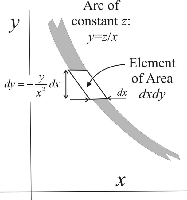
Starting with [math]\displaystyle{ y= \frac{z}{x} }[/math], we have [math]\displaystyle{ dy = -\frac{z}{x^2} \, dx = -\frac{y}{x} \, dx }[/math]. So the probability increment is [math]\displaystyle{ \delta p = f(x,y) \,dx\,|dy| = f_X(x)f_Y(z/x) \frac {y}{|x|} \, dx \, dx }[/math]. Since [math]\displaystyle{ z=yx }[/math] implies [math]\displaystyle{ dz=y\,dx }[/math], we can relate the probability increment to the [math]\displaystyle{ z }[/math]-increment, namely [math]\displaystyle{ \delta p = f_X(x)f_Y(z/x) \frac {1}{|x|} \, dx \, dz }[/math]. Then integration over [math]\displaystyle{ x }[/math], yields [math]\displaystyle{ f_Z(z)=\int f_X(x)f_Y(z/x) \frac {1}{|x| } \, dx }[/math].
2.3. A Bayesian Interpretation
Let [math]\displaystyle{ X \sim f(x) }[/math] be a random sample drawn from probability distribution [math]\displaystyle{ f_x(x) }[/math]. Scaling [math]\displaystyle{ X }[/math] by [math]\displaystyle{ \theta }[/math] generates a sample from scaled distribution [math]\displaystyle{ \theta X \sim \frac {1}{| \theta |} f_x \left ( \frac{x}{ \theta} \right ) }[/math] which can be written as a conditional distribution [math]\displaystyle{ g_x(x| \theta)= \frac {1}{| \theta |} f_x \left ( \frac {x}{ \theta } \right ) }[/math].
Letting [math]\displaystyle{ \theta }[/math] be a random variable with pdf [math]\displaystyle{ f_\theta ( \theta ) }[/math], the distribution of the scaled sample becomes [math]\displaystyle{ f_X ( \theta x ) = g_X(x\mid \theta) f_\theta (\theta) }[/math] and integrating out [math]\displaystyle{ \theta }[/math] we get [math]\displaystyle{ h_x(x) = \int_{-\infty}^\infty g_X(x| \theta) f_\theta (\theta) d\theta }[/math] so [math]\displaystyle{ \theta X }[/math] is drawn from this distribution [math]\displaystyle{ \theta X \sim h_X(x) }[/math]. However, substituting the definition of [math]\displaystyle{ g }[/math] we also have [math]\displaystyle{ h_X(x) = \int_{-\infty}^\infty \frac{1}{| \theta |} f_x \left ( \frac {x}{ \theta } \right ) f_\theta (\theta) \, d\theta }[/math] which has the same form as the product distribution above. Thus the Bayesian posterior distribution [math]\displaystyle{ h_X(x) }[/math] is the distribution of the product of the two independent random samples [math]\displaystyle{ \theta }[/math] and [math]\displaystyle{ X }[/math].
For the case of one variable being discrete, let [math]\displaystyle{ \theta }[/math] have probability [math]\displaystyle{ P_i }[/math] at levels [math]\displaystyle{ \theta_i }[/math] with [math]\displaystyle{ \sum_i P_i = 1 }[/math]. The conditional density is [math]\displaystyle{ f_X ( x \mid \theta_i ) = \frac {1}{| \theta_i |} f_x \left ( \frac{x}{ \theta_i} \right ) }[/math]. Therefore [math]\displaystyle{ f_X ( \theta x ) = \sum \frac {P_i}{| \theta_i |} f_X \left ( \frac{x}{ \theta_i} \right ) }[/math].
3. Expectation of Product of Random Variables
When two random variables are statistically independent, the expectation of their product is the product of their expectations. This can be proved from the Law of total expectation:
- [math]\displaystyle{ \operatorname{E}(X Y) = \operatorname{E}_Y ( \operatorname{E}_{X Y \mid Y} (X Y \mid Y)) }[/math]
In the inner expression, Y is a constant. Hence:
- [math]\displaystyle{ \operatorname{E}_{X Y \mid Y} (X Y \mid Y) = Y\cdot \operatorname{E}_{X\mid Y}[X] }[/math]
- [math]\displaystyle{ \operatorname{E}(X Y) = \operatorname{E}_Y ( Y\cdot \operatorname{E}_{X\mid Y}[X]) }[/math]
This is true even if X and Y are statistically dependent in which case [math]\displaystyle{ \operatorname{E}_{X\mid Y}[X] }[/math] is a function of Y. In the special case in which X and Y are statistically independent, it is a constant independent of Y. Hence:
- [math]\displaystyle{ \operatorname{E}(X Y) = \operatorname{E}_Y ( Y\cdot \operatorname{E}_{X}[X]) }[/math]
- [math]\displaystyle{ \operatorname{E}(X Y) = \operatorname{E}_X(X) \cdot \operatorname{E}_Y(Y) }[/math]
4. Variance of the Product of Independent Random Variables
Let [math]\displaystyle{ X, Y }[/math] be uncorrelated random variables with means [math]\displaystyle{ \mu_X, \mu_Y, }[/math] and variances [math]\displaystyle{ \sigma_X^2, \sigma_Y^2 }[/math]. The variance of the product XY is
- [math]\displaystyle{ \operatorname{Var}(XY) = (\sigma_X^2 + \mu_X^2 )(\sigma_Y^2 + \mu_Y^2 ) -\mu_X^2 \mu_Y^2 }[/math]
In the case of the product of more than two variables, if [math]\displaystyle{ X_1 \cdots X_n, \;\; n\gt 2 }[/math] are statistically independent then[4] the variance of their product is
- [math]\displaystyle{ \operatorname{Var}(X_1X_2\cdots X_n) = \prod_{i=1}^n (\sigma_i^2 + \mu_i^2 ) -\prod_{i=1}^n \mu_i^2 }[/math]
5. Characteristic Function of Product of Random Variables
Assume X, Y are independent random variables. The characteristic function of X is [math]\displaystyle{ \varphi_X(t) }[/math], and the distribution of Y is known. Then from the law of total expectation, we have[5]
- [math]\displaystyle{ \begin{align} \varphi_Z(t) & =\operatorname{E}(e^{itX Y}) \\ & = \operatorname{E}_Y ( \operatorname{E}_{X Y \mid Y} (e^{itX Y} \mid Y)) \\ & = \operatorname{E}_Y ( \operatorname{E}_{X \mid Y} (e^{itX Y} \mid Y)) \\ & = \operatorname{E}_Y ( \varphi_X(tY)) \end{align} }[/math]
If the characteristic functions and distributions of both X and Y are known, then alternatively, [math]\displaystyle{ \varphi_Z(t) = \operatorname{E}_X ( \varphi_Y(tX)) }[/math] also holds.
6. Mellin Transform
The Mellin transform of a distribution [math]\displaystyle{ f(x) }[/math] with support only on [math]\displaystyle{ x \ge 0 }[/math] and having a random sample [math]\displaystyle{ X }[/math] is
- [math]\displaystyle{ \mathcal{M}f(x) = \varphi(s)=\int_0^\infty x^{s-1} f(x) \, dx = \operatorname{E}[ X^{s-1}]. }[/math]
The inverse transform is
- [math]\displaystyle{ \mathcal{M}^{-1}\varphi (s) = f(x)=\frac{1}{2 \pi i} \int_{c-i \infty}^{c+i \infty} x^{-s} \varphi(s)\, ds. }[/math]
if [math]\displaystyle{ X \text{ and } Y }[/math] are two independent random samples from different distributions, then the Mellin transform of their product is equal to the product of their Mellin transforms:
- [math]\displaystyle{ \mathcal{M}_{XY}(s) = \mathcal{M}_X(s)\mathcal{M}_Y(s) }[/math]
If s is restricted to integer values, a simpler result is
- [math]\displaystyle{ \operatorname{E}[(XY)^n] = \operatorname{E}[X^n] \; \operatorname{E}[Y^n] }[/math]
Thus the moments of the random product [math]\displaystyle{ XY }[/math] are the product of the corresponding moments of [math]\displaystyle{ X \text{ and } Y }[/math] and this extends to non-integer moments, for example
- [math]\displaystyle{ \operatorname{E}[\sqrt[p] {XY}] = \operatorname{E}[\sqrt[p] X] \; \operatorname{E}[\sqrt[p] Y] }[/math].
The pdf of a function can be reconstructed from its moments using the saddlepoint approximation method.
A further result is that for independent X, Y
- [math]\displaystyle{ \operatorname{E}[X^pY^q] = \operatorname{E}[X^p] \operatorname{E}[Y^q] }[/math]
Gamma distribution example To illustrate how the product of moments yields a much simpler result than finding the moments of the distribution of the product, let [math]\displaystyle{ X,Y }[/math] be sampled from two Gamma distributions, [math]\displaystyle{ \Gamma(\theta)^{-1} x^{ \theta -1} e^{-x} }[/math] with parameters [math]\displaystyle{ \theta = \alpha, \beta }[/math] whose moments are
- [math]\displaystyle{ \operatorname{E}[X^p] = \int_0^\infty x^p \Gamma (x, \theta)\,dx = \frac {\Gamma(\theta+p)}{\Gamma(\theta) }. }[/math]
Multiplying the corresponding moments gives the Mellin transform result
- [math]\displaystyle{ \operatorname{E}[(XY)^p] = \operatorname{E}[X^p] \; \operatorname{E}[Y^p] = \frac{ \Gamma(\alpha+p)}{\Gamma(\alpha)} \; \frac{ \Gamma(\beta+p)}{\Gamma(\beta)} }[/math]
Independently, it is known that the product of two independent Gamma samples has the distribution
- [math]\displaystyle{ f(z,\alpha,\beta) = 2 \Gamma(\alpha)^{-1} \Gamma(\beta)^{-1}z^{\frac{\alpha+\beta}{2}-1}K_{\alpha-\beta}(2\sqrt z), \; z\ge 0 }[/math].
To find the moments of this, make the change of variable [math]\displaystyle{ y = 2 \sqrt z }[/math], simplifying similar integrals to:
- [math]\displaystyle{ \int_0^\infty z^p K_\nu (2 \sqrt z) \, dz = 2^{-2p-1} \int_0^\infty y^{2p+1} K_\nu (y) \, dy }[/math]
thus
- [math]\displaystyle{ 2 \int_0^\infty z^{\frac{\alpha+\beta}{2}-1} K_{\alpha-\beta} (2 \sqrt z) \, dz = 2^{-(\alpha+\beta) - 2p+1} \int_0^{\infty} y^{(\alpha+\beta) + 2p -1} K_{\alpha-\beta}(y) \, dy }[/math]
The definite integral
- [math]\displaystyle{ \int_0^{\infty} y^\mu K_\nu (y) \,dy = 2^{\mu -1} \Gamma \left ( \frac{1+ \mu + \nu}{2} \right ) \Gamma \left (\frac{1+ \mu - \nu}{2} \right ) }[/math] is well documented and we have finally
- [math]\displaystyle{ \begin{align} E[Z^p] & = \frac {2^{-(\alpha+\beta) - 2p+1} \; 2^{(\alpha+\beta) + 2p -1} }{\Gamma(\alpha) \; \Gamma(\beta)} \Gamma \left ( \frac{(\alpha+\beta+2p)+(\alpha-\beta)}{2} \right ) \Gamma \left( \frac{(\alpha+\beta+2p)-(\alpha-\beta)}{2} \right ) \\ \\ & = \frac{\Gamma( \alpha+ p) \, \Gamma(\beta + p)} {\Gamma(\alpha) \, \Gamma(\beta)} \end{align} }[/math]
which, after some difficulty, has agreed with the moment product result above.
If X, Y are drawn independently from Gamma distributions with shape parameters [math]\displaystyle{ \alpha, \; \beta }[/math] then
- [math]\displaystyle{ \operatorname{E}[X^pY^q] = \operatorname{E}[X^p] \; \operatorname{E}[Y^q] = \frac{ \Gamma(\alpha+p)}{\Gamma(\alpha)} \; \frac{ \Gamma(\beta+q)}{\Gamma(\beta)} }[/math]
This type of result is universally true, since for bivariate independent variables [math]\displaystyle{ f_{x,y}(x,y) = f_X(x) f_Y(y) }[/math] thus
- [math]\displaystyle{ \begin{align} \operatorname{E}[X^pY^q] & = \int_{x=-\infty}^\infty \int_{y=-\infty}^\infty x^p y^q f_{x,y}(x,y) \, dy \, dx \\ & = \int_{x=-\infty}^\infty x^p \Big [ \int_{y=-\infty}^\infty y^q f_Y(y)\, dy \Big ] f_X(x) \, dx \\ & = \int_{x=-\infty}^\infty x^p f_X(x) \, dx \int_{y=-\infty}^{\infty} y^q f_Y(y) \, dy \\ & = \operatorname{E}[X^p] \; \operatorname{E}[Y^q] \end{align} }[/math]
or equivalently it is clear that [math]\displaystyle{ X^p \text{ and } Y^q }[/math] are independent variables.
7. Special Cases
7.1. Lognormal Distributions
The distribution of the product of two random variables which have lognormal distributions is again lognormal. This is itself a special case of a more general set of results where the logarithm of the product can be written as the sum of the logarithms. Thus, in cases where a simple result can be found in the list of convolutions of probability distributions, where the distributions to be convolved are those of the logarithms of the components of the product, the result might be transformed to provide the distribution of the product. However this approach is only useful where the logarithms of the components of the product are in some standard families of distributions.
7.2. Uniformly Distributed Independent Random Variables
Let [math]\displaystyle{ Z }[/math] be the product of two independent variables [math]\displaystyle{ Z= X_1 X_2 }[/math] each uniformly distributed on the interval [0,1], possibly the outcome of a copula transformation. As noted in "Lognormal Distributions" above, PDF convolution operations in the Log domain correspond to the product of sample values in the original domain. Thus, making the transformation [math]\displaystyle{ u=\ln (x) }[/math], such that [math]\displaystyle{ p_U(u) \, |du| = p_X(x) \, |dx| }[/math], each variate is distributed independently on u as
- [math]\displaystyle{ p_U (u) = p_X(x) / |du/dx| = \frac {1}{x^{-1}} = e^u, \;\; -\infty \lt u \le 0 }[/math].
and the convolution of the two distributions is the autoconvolution
- [math]\displaystyle{ c(y) = \int_{u=0}^y e^u e^{y-u} du = - \int_{u=y}^0 e^y du = -y e^y , \;\; -\infty \lt y \le 0 }[/math]
Next retransform the variable to [math]\displaystyle{ z=e^y }[/math] yielding the distribution
- [math]\displaystyle{ c_2(z) = c_Y(y)/|dz/dy| = \frac {-y e^y }{e^y} = -y = \ln (1/z) }[/math] on the interval [0,1]
For the product of multiple ( >2 ) independent samples the characteristic function route is favorable. If we define [math]\displaystyle{ \tilde{y} = -y }[/math] then [math]\displaystyle{ c(\tilde{y}) }[/math] above is a Gamma distribution of shape 1 and scale factor 1, [math]\displaystyle{ c(\tilde{y}) = \tilde{y} e^{-\tilde{y}} }[/math] , and its known CF is [math]\displaystyle{ (1 - i t)^{-1} }[/math]. Note that [math]\displaystyle{ |d\tilde{y}| = |dy| }[/math] so the Jacobian of the transformation is unity.
The convolution of [math]\displaystyle{ n }[/math] independent samples from [math]\displaystyle{ \tilde{Y} }[/math] therefore has CF [math]\displaystyle{ (1 - i t)^{-n} }[/math] which is known to be the CF of a Gamma distribution of shape [math]\displaystyle{ n }[/math]:
- [math]\displaystyle{ c_n (\tilde{y}) = \Gamma(n)^{-1} \tilde{y}^{(n-1)} e^{-\tilde{y}} = \Gamma(n)^{-1} (-y)^{(n-1)} e^y }[/math].
Making the inverse transformation [math]\displaystyle{ z=e^y }[/math] we get the PDF of the product of the n samples:
- [math]\displaystyle{ f_n(z) = \frac {c_n(y)}{|dz/dy|} = \Gamma(n)^{-1} \Big (-\log z \Big )^{n-1} e^y / e^y = \frac{\Big (-\log z \Big )^{n-1} }{(n-1)! \;\;\;} }[/math]
The following, more conventional, derivation from Stackexchange[6] is consistent with this result. First of all, letting [math]\displaystyle{ Z_2 = X_1 X_2 }[/math] its CDF is
- [math]\displaystyle{ \begin{align} F_{Z_2}(z) = \Pr \Big [ Z_2 \le z \Big ] & = \int_{x=0}^1 \Pr \Big [ X_2 \le \frac{z}{x} \Big ] f_{X_1} (x) \, dx \\ & = \int_{x=0}^z dx + \int_{x=z}^1 \frac{z}{x} \, dx \\ & = z - z\log z, \;\; 0 \lt z \le 1 \end{align} }[/math]
The density of [math]\displaystyle{ z_2 \text{ is then } f(z_2) = -\log(z_2) }[/math]
Multiplying by a third independent sample gives distribution function
- [math]\displaystyle{ \begin{align} F_{Z_3}(z) = \Pr \Big [Z_3 \le z \Big ] & = \int_{x=0}^1 \Pr \Big [ X_3 \le \frac{z}{x} \Big] f_{Z_2}(x) \, dx \\ & = -\int_{x=0}^z \log(x) \, dx - \int_{x=z}^1 \frac{z}{x} \log(x) \,dx \\ & = -z \Big (\log(z) - 1 \Big ) + \frac{1}{2}z \log^2 (z) \end{align} }[/math]
Taking the derivative yields [math]\displaystyle{ f_{Z_3}(z) = \frac{1}{2} \log^2 (z), \;\; 0 \lt z \le 1. }[/math]
The author of the note conjectures that, in general, [math]\displaystyle{ f_{Z_n}(z) = \frac{( - \log z )^{n-1} }{ (n-1)! \;\;\;}, \;\; 0 \lt z \le 1 }[/math]
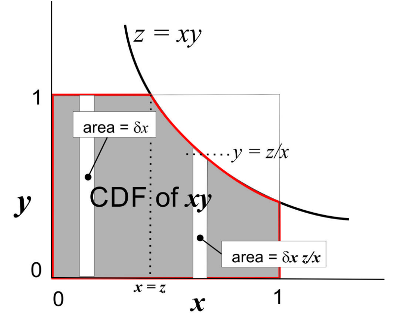
The figure illustrates the nature of the integrals above. The shaded area within the unit square and below the line z = xy, represents the CDF of z. This divides into two parts. The first is for 0 < x < z where the increment of area in the vertical slot is just equal to dx. The second part lies below the xy line, has y-height z/x, and incremental area dx z/x.
7.3. Independent Central-Normal Distributions
The product of two independent Normal samples follows a modified Bessel function. Let [math]\displaystyle{ x, y }[/math] be samples from a Normal(0,1) distribution and [math]\displaystyle{ z=xy }[/math]. Then
- [math]\displaystyle{ p_Z(z) = \frac {K_0(|z|)}{\pi}, \;\;\; -\infty \lt z \lt +\infty }[/math]
The variance of this distribution could be determined, in principle, by a definite integral from Gradsheyn and Ryzhik,[7]
- [math]\displaystyle{ \int_0^\infty x^\mu K_\nu (ax) \, dx = 2^{\mu - 1} a^{-\mu - 1} \Gamma \Big ( \frac{1 + \mu + \nu}{2} \Big ) \Gamma \Big ( \frac{1 + \mu - \nu}{2} \Big), \;\; a\gt 0, \;\nu + 1 \pm \mu \gt 0 }[/math]
thus [math]\displaystyle{ \int_{-\infty}^\infty \frac{z^2 K_0 (|z|)}{\pi} \, dz = \frac{4}{\pi} \; \Gamma^2 \Big (\frac{3}{2} \Big ) = 1 }[/math]
A much simpler result, stated in a section above, is that the variance of the product of zero-mean independent samples is equal to the product of their variances. Since the variance of each Normal sample is one, the variance of the product is also one.
The product of correlated Normal samples case was recently addressed by Nadarajaha and Pogány.[8] Let [math]\displaystyle{ X \text{, } Y }[/math] be zero mean, unit variance, normally distributed variates with correlation coefficient [math]\displaystyle{ \rho \text { and let } Z = XY }[/math]
Then
- [math]\displaystyle{ f_Z(z) = \frac{1}{\pi \sqrt{1-\rho^2} }\exp \left ( \frac{ \rho z}{ 1 - \rho^2 } \right ) K_0 \left ( \frac{|z| }{ 1 - \rho^2 } \right ) }[/math]
Mean and variance: For the mean we have [math]\displaystyle{ \operatorname{E}[Z] = \rho }[/math] from the definition of correlation coefficient. The variance can be found by transforming from two unit variance zero mean uncorrelated variables U, V. Let
- [math]\displaystyle{ X = U, \;\; Y = \rho U + \sqrt{(1-\rho^2)} V }[/math]
Then X, Y are unit variance variables with correlation coefficient [math]\displaystyle{ \rho }[/math] and
- [math]\displaystyle{ (XY)^2 = U^2 \bigg ( \rho U + \sqrt {(1-\rho^2)}V \bigg )^2 = U^2 \bigg (\rho^2 U^2 + 2\rho \sqrt{1-\rho^2}UV + (1-\rho^2) V^2 \bigg ) }[/math]
Removing odd-power terms, whose expectations are obviously zero, we get
- [math]\displaystyle{ \operatorname{E}[(XY)^2] = \rho^2\operatorname{E}[U^4] + (1-\rho^2)\operatorname{E}[U^2]\operatorname{E}[V^2] = 3 \rho^2 + (1-\rho^2) = 1 + 2 \rho^2 }[/math]
Since [math]\displaystyle{ (\operatorname{E}[Z])^2 = \rho^2 }[/math] we have
-
- [math]\displaystyle{ \operatorname{Var}(Z) = \operatorname{E}[Z^2] - (\operatorname{E}[Z])^2= 1 + 2 \rho^2 - \rho^2 = 1 + \rho^2 }[/math]
High correlation asymptote In the highly correlated case, [math]\displaystyle{ \rho \rightarrow 1 }[/math] the product converges on the square of one sample. In this case the [math]\displaystyle{ K_0 }[/math] asymptote is [math]\displaystyle{ K_0(x) \rightarrow \sqrt{\tfrac{\pi}{2x} } e^{-x} \text{ in the limit as } x = \frac {|z|}{1-\rho^2} \rightarrow \infty }[/math] and
- [math]\displaystyle{ \begin{align} p(z) & \rightarrow \frac{1}{\pi \sqrt{1-\rho^2} } \exp \left (\frac{\rho z}{1-\rho^2 } \right) \sqrt{\frac{\pi (1-\rho^2)}{2z} } \exp\left (-\frac{|z|}{1-\rho^2} \right) \\ & = \frac{1}{\sqrt{2\pi z } } \exp \Bigg (\frac{ -|z| +\rho z}{(1-\rho)(1+\rho) } \Bigg) \\ & = \frac{1}{\sqrt{2\pi z } } \exp \Bigg (\frac{ -z }{1+\rho } \Bigg), \;\; z\gt 0 \\ & \rightarrow \frac{1}{\Gamma(\tfrac{1}{2})\sqrt{2 z } } e^{-\tfrac{ z }{2 } }, \;\; \text { as }\rho \rightarrow 1 \\ \end{align} }[/math]
which is a Chi-squared distribution with one degree of freedom.
Multiple correlated samples. Nadarajaha et. al. further show that if [math]\displaystyle{ Z_1, Z_2,..Z_n \text{ are } n }[/math] iid random variables sampled from [math]\displaystyle{ f_Z(z) }[/math] and [math]\displaystyle{ \bar{Z} = \tfrac{1}{n} \sum Z_i }[/math] is their mean then
- [math]\displaystyle{ f_\bar Z( z)= \frac {n^{n/2} 2^{-n/2} } { \Gamma (\frac {n}{2} ) } |z|^{n/2-1 } \exp \left( \frac{\beta-\gamma}{2}z \right) {W}_{0,\frac{1-n}{2}}(| z |), \;\; -\infty \lt z \lt \infty. }[/math]
where W is the Whittaker function while [math]\displaystyle{ \beta = \frac{n}{1 - \rho}, \;\; \gamma = \frac{n}{1 + \rho} }[/math].
Using the identity [math]\displaystyle{ W_{0,\nu}(x)= \sqrt {\frac{x}{\pi}}K_\nu(x/2), \;\; x \ge 0 }[/math], see for example the DLMF compilation. eqn(13.13.9),[9] this expression can be somewhat simplified to
- [math]\displaystyle{ f_\bar z( z)= \frac {n^{n/2} 2^{-n/2} } { \Gamma (\frac {n}{2} ) } |z|^{n/2-1 } \exp \left (\frac{\beta-\gamma}{2}z \right ) \sqrt{ \frac{ \beta+\gamma }{\pi} |z| } \; K_{ \frac {1-n}{2}} \left ( \frac{\beta+\gamma}{2} |z| \right ), \;\; -\infty \lt z \lt \infty. }[/math]
The pdf gives the distribution of a sample covariance.
Multiple non-central correlated samples. The distribution of the product of correlated non-central normal samples was derived by Cui et.al.[10] and takes the form of an infinite series of modified Bessel functions of the first kind.
Moments of product of correlated central normal samples
For a central normal distribution N(0,1) the moments are
- [math]\displaystyle{ \operatorname{E}\left[X^p\right] = \frac{1}{\sigma \sqrt{2\pi}}\int_{-\infty}^{\infty} x^p \exp (-\tfrac {x^2}{2\sigma^2}) \, dx= \begin{cases} 0 & \text{if }p\text{ is odd,} \\ \sigma^p (p-1)!! & \text{if }p\text{ is even.} \end{cases} }[/math]
where [math]\displaystyle{ n!! }[/math] denotes the double factorial.
If [math]\displaystyle{ X,Y \sim \text{Norm}(0,1) }[/math] are central correlated variables, the simplest bivariate case of the multivariate normal moment problem described by Kan,[11] then
- [math]\displaystyle{ \operatorname{E}[X^pY^q] = \begin{cases} 0 & \text{if }p+q \text{ is odd,} \\ \frac {p!q!}{2^{\tfrac{p+q}{2} } }\sum_{k=0}^t \frac { (2\rho)^{2k} }{\Big(\frac{p}{2}- k \Big)! \; \Big(\frac{q}{2}- k \Big)! \;(2k)! } & \text{if } p \text{ and } q \text{ are even} \\ \frac {p!q!}{2^{\tfrac{p+q}{2} } }\sum_{k=0}^t \frac { (2\rho)^{2k+1} }{\Big(\frac{p-1}{2}- k \Big)! \; \Big(\frac{q-1}{2}- k \Big)! \; (2k+1)! } & \text{if } p \text{ and } q \text{ are odd} \end{cases} }[/math]
where
- [math]\displaystyle{ \rho }[/math] is the correlation coefficient and [math]\displaystyle{ t = \min([p,q]/2) }[/math]
[needs checking]
The distribution of the product of non-central correlated normal samples was derived by Cui et al.[10] and takes the form of an infinite series.
These product distributions are somewhat comparable to the Wishart distribution. The latter is the joint distribution of the four elements (actually only three independent elements) of a sample covariance matrix. If [math]\displaystyle{ x_t, y_t }[/math] are samples from a bivariate time series then the [math]\displaystyle{ W = \sum_{t=1}^K \dbinom {x_t}{y_t} {\dbinom {x_t}{y_t} }^T }[/math] is a Wishart matrix with K degrees of freedom. The product distributions above are the unconditional distribution of the aggregate of K > 1 samples of [math]\displaystyle{ W_{2,1} }[/math].
7.6. Independent Complex-Valued Central-Normal Distributions
Let [math]\displaystyle{ u_1, v_1, u_2, v_2 }[/math] be independent samples from a normal(0,1) distribution.
Setting [math]\displaystyle{ z_1 = u_1 + i v_1 \text{ and } z_2 = u_2 + i v_2 \text{ then } z_1, z_2 }[/math] are independent zero-mean complex normal samples with circular symmetry. Their complex variances are [math]\displaystyle{ \operatorname{Var} |z_i| = 2. }[/math]
The density functions of
- [math]\displaystyle{ r_i \equiv |z_i| = (u_i^2 + v_i^2)^{\frac{1}{2}}, \;\;i=1,2 }[/math] are Rayleigh distributions defined as:
- [math]\displaystyle{ f_r(r_i) = r_i e^{-r_i^2 / 2} \text{ of mean } \sqrt{\tfrac{\pi}{2}} \text{ and variance} \frac{4-\pi}{2} }[/math]
The variable [math]\displaystyle{ y_i \equiv r_i^2 }[/math] is clearly Chi-squared with two degrees of freedom and has PDF
- [math]\displaystyle{ f_{y_i}(y_i) = \tfrac{1}{2} e^{-y_i/2} \text{ of mean value } 2 }[/math]
Wells et. al.[12] show that the density function of [math]\displaystyle{ s \equiv |z_1 z_2| }[/math] is
- [math]\displaystyle{ f_s (s) = s K_0(s), \;\; s \ge 0 }[/math]
and the cumulative distribution function of [math]\displaystyle{ s }[/math] is
- [math]\displaystyle{ P(a) = \Pr [s \le a ] = \int_{s=0}^a s K_0(s) ds = 1 - a K_1(a) }[/math]
Thus the polar representation of the product of two uncorrelated complex Gaussian samples is
- [math]\displaystyle{ f_{s,\theta}(s,\theta) = f_s(s) p_\theta(\theta) \text{ where } p(\theta) \text{ is uniform on }[0,2\pi] }[/math].
The first and second moments of this distribution can be found from the integral in Normal Distributions above
- [math]\displaystyle{ m_1 = \int_0^\infty s^2 K_0 (s) \, dx = 2 \Gamma^2 ( \tfrac{3}{2} ) = 2 (\tfrac {\sqrt \pi}{2})^2 = \frac{\pi}{2} }[/math]
- [math]\displaystyle{ m_2 = \int_0^\infty s^3 K_0 (s) \, dx = 2^2 \Gamma^2 ( \tfrac{4}{2} ) = 4 }[/math]
Thus its variance is [math]\displaystyle{ \operatorname{Var} (s) = m_2 - m_1^2 = 4 - \frac{\pi^2}{4} }[/math].
Further, the density of [math]\displaystyle{ z \equiv s^2 = {|r_1 r_2|}^2 = {|r_1 |}^2 {| r_2|}^2 = y_1 y_2 }[/math] corresponds to the product of two independent Chi-square samples [math]\displaystyle{ y_i }[/math] each with two DoF. Writing these as scaled Gamma distributions [math]\displaystyle{ f_y(y_i) = \tfrac{1}{\theta \Gamma(1) } e^{-y_i/\theta } \text{ with } \theta = 2 }[/math] then, from the Gamma products below, the density of the product is
- [math]\displaystyle{ f_Z(z) = \tfrac{1}{2} K_0(\sqrt{z}) \text{ with expectation } \operatorname{E}(z) = 4 }[/math]
7.7. Independent Complex-Valued Noncentral Normal Distributions
The product of non-central independent complex Gaussians is described by O’Donoughue and Moura[13] and forms a double infinite series of modified Bessel functions of the first and second types.
7.8. Gamma Distributions
The product of two independent Gamma samples, [math]\displaystyle{ z = x_1 x_2 }[/math], defining [math]\displaystyle{ \Gamma(x;k_i,\theta_i) = \frac {x^{k_i-1}e^{-x/\theta_i}}{\Gamma(k_i) \theta_i^{k_i} } }[/math], follows[14]
- [math]\displaystyle{ \begin{align} p_Z(z) & = \frac {2}{\Gamma(k_1) \Gamma(k_2) } \frac { z ^{\frac {k_1 + k_2}{2 } -1} } { \left(\theta_1 \theta_2 \right) ^{\frac {k_1 + k_2}{2 }} } K_{k_1 -k_2 } \left( 2 \sqrt{ \frac {z}{\theta_1 \theta_2} } \right) \\ \\ & = \frac {2}{\Gamma(k_1) \Gamma(k_2) } \frac {y^{\frac {k_1 + k_2}{2 }-1}} {\theta_1 \theta_2 } K_{k_1 -k_2 } \left(2 \sqrt y \right) \text { where } y = \frac {z}{\theta_1 \theta_2}\\ \end{align} }[/math]
7.9. Beta Distributions
Nagar et. al.[15] define a correlated bivariate beta distribution
- [math]\displaystyle{ f(x,y) = \frac {x^{a-1}y^{b-1}(1-x)^{b+c-1}(1-y)^{a+c-1} } {B(a,b,c) (1-xy)^{a+b+c} }, \;\;\;0\lt x,y \lt 1 }[/math]
where
- [math]\displaystyle{ B(a,b,c) = \frac {\Gamma(a) \Gamma(b) \Gamma(c)}{ \Gamma(a+b+c) } }[/math]
Then the pdf of Z = XY is given by
- [math]\displaystyle{ f_Z(z) = \frac {B(a+c,b+c) z^{a-1} (1-z)^{c-1} } {B(a,b,c) } {_2F_1} (a+c,a+c; a+b+2c; 1-z), \;\;\; 0\lt z \lt 1 }[/math]
where [math]\displaystyle{ {_2F_1} }[/math] is the Gauss hypergeometric function defined by the Euler integral
- [math]\displaystyle{ {_2F_1}(a,b,c,z) = \frac {\Gamma(c) }{\Gamma(a) \Gamma (c-a) } \int_0^1 v^{a-1} (1-v)^{c-a-1} (1-vz)^{-b} \, dv }[/math]
Note that multivariate distributions are not generally unique, apart from the Gaussian case, and there may be alternatives.
7.10. Uniform and Gamma Distributions
The distribution of the product of a random variable having a uniform distribution on (0,1) with a random variable having a gamma distribution with shape parameter equal to 2, is an exponential distribution.[16] A more general case of this concerns the distribution of the product of a random variable having a beta distribution with a random variable having a gamma distribution: for some cases where the parameters of the two component distributions are related in a certain way, the result is again a gamma distribution but with a changed shape parameter.[16]
The K-distribution is an example of a non-standard distribution that can be defined as a product distribution (where both components have a gamma distribution).
7.11. Gamma and Pareto Distributions
The product of n Gamma and m Pareto independent samples was derived by Nadarajah.[17]
8. In Theoretical Computer Science
In computational learning theory, a product distribution [math]\displaystyle{ \mathcal{D} }[/math] over [math]\displaystyle{ \{0,1\}^n }[/math] is specified by the parameters [math]\displaystyle{ \mu_1, \mu_2, \dots, \mu_n }[/math]. Each parameter [math]\displaystyle{ \mu_i }[/math] gives the marginal probability that the ith bit of [math]\displaystyle{ x \in \{0,1\}^n }[/math] sampled as [math]\displaystyle{ x \sim \mathcal{D} }[/math] is 1; i.e. [math]\displaystyle{ \mu_i = \Pr_{\mathcal{D}}[x_i = 1] }[/math]. In this setting, the uniform distribution is simply a product distribution with every [math]\displaystyle{ \mu_i = 1/2 }[/math].
Product distributions are a key tool used for proving learnability results when the examples cannot be assumed to be uniformly sampled.[18] They give rise to an inner product [math]\displaystyle{ \langle \cdot, \cdot \rangle }[/math] on the space of real-valued functions on [math]\displaystyle{ \{0,1\}^n }[/math] as follows:
- [math]\displaystyle{ \langle f, g \rangle_\mathcal{D} = \sum_{x \in \{0,1\}^n} \mathcal{D}(x)f(x)g(x) = \mathbb{E}_{\mathcal{D}} [fg] }[/math]
This inner product gives rise to a corresponding norm as follows:
- [math]\displaystyle{ \|f\|_{\mathcal{D}} = \sqrt{ \langle f, f \rangle_\mathcal{D} } }[/math]
The content is sourced from: https://handwiki.org/wiki/Product_distribution
References
- Springer, Melvin Dale (1979). The Algebra of Random Variables. John Wiley & Sons. ISBN 978-0-471-01406-5. https://archive.org/details/algebraofrandomv0000spri. Retrieved 24 September 2012.
- Rohatgi, V. K. (1976). An Introduction to Probability Theory and Mathematical Statistics. Wiley Series in Probability and Statistics. New York: Wiley. doi:10.1002/9781118165676. ISBN 978-0-19-853185-2. https://dx.doi.org/10.1002%2F9781118165676
- Grimmett, G. R.; Stirzaker, D.R. (2001). Probability and Random Processes. Oxford: Oxford University Press. ISBN 978-0-19-857222-0. http://ukcatalogue.oup.com/product/9780198572220.do?keyword=grimmett+stirzaker&sortby=bestMatches. Retrieved 4 October 2015.
- Sarwate, Dilip (March 9, 2013). "Variance of product of multiple random variables". Stack Exchange. https://stats.stackexchange.com/q/52699.
- "How to find characteristic function of product of random variables". Stack Exchange. January 3, 2013. https://math.stackexchange.com/q/269579.
- heropup (1 February 2014). "product distribution of two uniform distribution, what about 3 or more". Stack Exchange. https://math.stackexchange.com/q/659278.
- Gradsheyn, I S; Ryzhik, I M (1980). Tables of Integrals, Series and Products. Academic Press. pp. section 6.561.
- Nadarajah, Saralees; Pogány, Tibor (2015). "On the distribution of the product of correlated normal random variables". Comptes Rendus de l'Académie des Sciences, Série I 354 (2): 201–204. doi:10.1016/j.crma.2015.10.019. https://dx.doi.org/10.1016%2Fj.crma.2015.10.019
- Equ(13.18.9). "Digital Library of Mathematical Functions". https://dlmf.nist.gov.
- Cui, Guolong (2016). "Exact Distribution for the Product of Two Correlated Gaussian Random Variables". IEEE Signal Processing Letters 23 (11): 1662–1666. doi:10.1109/LSP.2016.2614539. Bibcode: 2016ISPL...23.1662C. https://dx.doi.org/10.1109%2FLSP.2016.2614539
- Kan, Raymond (2008). "From moments of sum to moments of product". Journal of Multivariate Analysis 99 (3): 542–554. doi:10.1016/j.jmva.2007.01.013. https://dx.doi.org/10.1016%2Fj.jmva.2007.01.013
- Wells, R T; Anderson, R L; Cell, J W (1962). "The Distribution of the Product of Two Central or Non-Central Chi-Square Variates". The Annals of Mathematical Statistics 33 (3): 1016–1020. doi:10.1214/aoms/1177704469. https://dx.doi.org/10.1214%2Faoms%2F1177704469
- O’Donoughue, N; Moura, J M F (March 2012). "On the Product of Independent Complex Gaussians". IEEE Transactions on Signal Processing 60 (3): 1050–1063. doi:10.1109/TSP.2011.2177264. Bibcode: 2012ITSP...60.1050O. https://dx.doi.org/10.1109%2FTSP.2011.2177264
- Wolfies (August 2017). "PDF of the product of two independent Gamma random variables". https://math.stackexchange.com/q/2396324.
- Nagar, D K; Orozco-Castañeda, J M; Gupta, A K (2009). "Product and quotient of correlated beta variables". Applied Mathematics Letters 22: 105–109. doi:10.1016/j.aml.2008.02.014. https://dx.doi.org/10.1016%2Fj.aml.2008.02.014
- Johnson, Norman L.; Kotz, Samuel; Balakrishnan, N. (1995). Continuous Univariate Distributions Volume 2, Second edition. Wiley. p. 306. ISBN 978-0-471-58494-0. http://www.wiley.com/WileyCDA/WileyTitle/productCd-0471584940.html. Retrieved 24 September 2012.
- Nadarajah, Saralees (June 2011). "Exact distribution of the product of n gamma and m Pareto random variables". Journal of Computational and Applied Mathematics 235 (15): 4496–4512. doi:10.1016/j.cam.2011.04.018. https://dx.doi.org/10.1016%2Fj.cam.2011.04.018
- Servedio, Rocco A. (2004), "On learning monotone DNF under product distributions", Information and Computation 193 (1): 57–74, doi:10.1016/j.ic.2004.04.003 https://dx.doi.org/10.1016%2Fj.ic.2004.04.003