1. Advantages

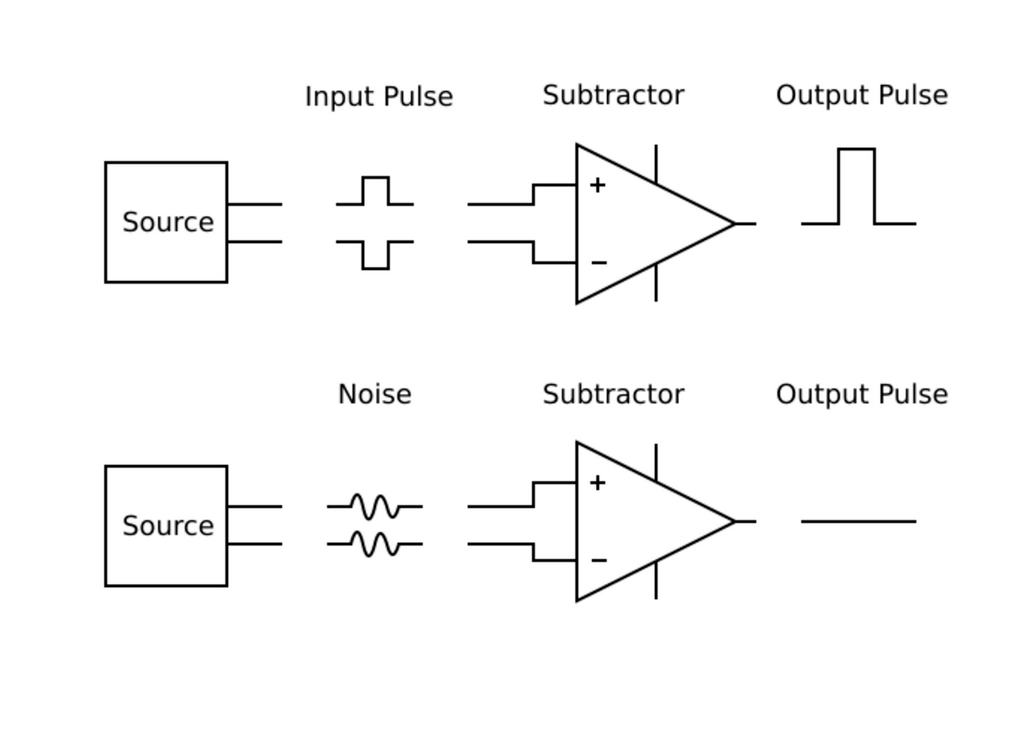
Provided that the impedances of two conductors in a circuit are equal (it is balanced), external electromagnetic interference tends to affect both conductors identically. Since the receiving circuit only detects the difference between the wires, the technique resists electromagnetic noise compared to one conductor with an un-balanced reference (low-Ω connection to ground).

Contrary to popular belief, differential signaling does not affect noise cancellation. Balanced lines with differential receivers will reject noise regardless of whether the signal is differential or single-ended, but since balanced line noise rejection requires a differential receiver anyway, differential signaling is often used on balanced lines. This improves SNR, reduces EMI, and makes the signal more immune to ground currents or differences.^[1]

The technique works for both analog signaling, as in balanced audio, and in digital signaling, as in RS-422, RS-485, Ethernet over twisted pair, PCI Express, DisplayPort, HDMI and USB.

In a system with a differential receiver, desired signals add and noise is subtracted away. https://handwiki.org/wiki/index.php?curid=2029472

1.1. Suitability for Use with Low-Voltage Electronics

The electronics industry, particularly in portable and mobile devices, continually strives to lower supply voltage to save power. A low supply voltage, however, reduces noise immunity. Differential signaling helps to reduce these problems because, for a given supply voltage, it provides twice the noise immunity of a single-ended system.

To see why, consider a single-ended digital system with supply voltage [math]\displaystyle{ V_S }[/math]. The high logic level is [math]\displaystyle{ V_S\, }[/math] and the low logic level is 0 V. The difference between the two levels is therefore [math]\displaystyle{ V_S - 0\,\mathrm{V} = V_S }[/math]. Now consider a differential system with the same supply voltage. The voltage difference in the high state, where one wire is at [math]\displaystyle{ V_S\, }[/math] and the other at 0 V, is [math]\displaystyle{ V_S - 0\,\mathrm{V} = V_S }[/math]. The voltage difference in the low state, where the voltages on the wires are exchanged, is [math]\displaystyle{ 0\,\mathrm{V} - V_S = -V_S }[/math]. The difference between high and low logic levels is therefore [math]\displaystyle{ V_S - (-V_S) = 2V_S\, }[/math]. This is twice the difference of the single-ended system. If the voltage noise on one wire is uncorrelated to the noise on the other one, it takes twice as much noise to cause an error with the differential system as with the single-ended system. In other words, differential signaling doubles the noise immunity.

1.2. Resistance to Electromagnetic Interference

This advantage is not directly due to differential signaling itself, but to the common practice of transmitting differential signals on balanced lines.^[2][3] Single-ended signals are still resistant to interference if the lines are balanced and terminated by a differential amplifier.

2. Comparison with Single-Ended Signaling

In single-ended signaling, the transmitter generates a single voltage that the receiver compares with a fixed reference voltage, both relative to a common ground connection shared by both ends. In many instances single-ended designs are not feasible. Another difficulty is the electromagnetic interference that can be generated by a single-ended signaling system that attempts to operate at high speed.

3. Generalization: Ensemble Signaling

The disadvantage of differential signal transmission is that it requires twice as many wires as single-ended signal transmission. Ensemble signaling improves this by using [math]\displaystyle{ n }[/math] wires to transmit [math]\displaystyle{ n-1 }[/math] differential signals. For [math]\displaystyle{ n = 2 }[/math], it is equivalent to differential signalling.

3.1. Two-Wire Ensemble Signalling

Two-wire ensemble signalling encodes one signal using two wires. On the encoder side, using the generator matrix

[math]\displaystyle{ \mathbf{G} := \begin{pmatrix} +1 & 1 \\ -1 & 1 \end{pmatrix} }[/math]

and the input vector [math]\displaystyle{ x := (x_1, x_2) }[/math] gives [math]\displaystyle{ y = \mathbf{G} \cdot x }[/math], the two signals to transmit.

On the decoder side, using the control matrix [math]\displaystyle{ \mathbf{H} := \mathbf{G}^{-1} }[/math]

[math]\displaystyle{ \mathbf{H} := \begin{pmatrix} +1/2 & -1/2 \\ \;\; 1/2 & \;\; 1/2 \end{pmatrix} }[/math]

and the input vector [math]\displaystyle{ y }[/math] gives the initial vector [math]\displaystyle{ x := \mathbf{H} \cdot y }[/math].

However, only [math]\displaystyle{ x_1 }[/math] is insensitive to common-mode interferences, while [math]\displaystyle{ x_2 }[/math] is highly sensitive to common-mode interferences. Removing [math]\displaystyle{ x_2 }[/math] from the calculation gives normal differential signaling:

[math]\displaystyle{ \mathbf{G} := \begin{pmatrix} +1 \\ -1 \end{pmatrix}\; }[/math] and [math]\displaystyle{ \; \mathbf{H} := \begin{pmatrix} +1/2 & -1/2 \\ \end{pmatrix} }[/math]

3.2. Four-Wire Ensemble Signalling

Four-wire ensemble signalling encodes three signals using four wires. On the encoder side, using the generator matrix

[math]\displaystyle{ \mathbf{G} := \begin{pmatrix} 1 & -1/3 & -1/3 & 1/3 \\ -1/3 & 1 & -1/3 & 1/3 \\ -1/3 & -1/3 & 1 & 1/3 \\ -1/3 & -1/3 & -1/3 & 1/3 \end{pmatrix} }[/math]

and the input vector [math]\displaystyle{ x := (x_1, x_2, x_3, x_4) }[/math] gives [math]\displaystyle{ y = \mathbf{G} \cdot x }[/math], the four signals to transmit.

On the decoder side, using the control matrix [math]\displaystyle{ \mathbf{H} := \mathbf{G}^{-1} }[/math]

[math]\displaystyle{ \mathbf{H} := \begin{pmatrix} 3/4 & 0 & 0 & -3/4 \\ 0 & 3/4 & 0 & -3/4 \\ 0 & 0 & 3/4 & -3/4 \\ 3/4 & 3/4 & 3/4 & 3/4 \end{pmatrix} }[/math]

and the input vector [math]\displaystyle{ y }[/math] gives the initial vector [math]\displaystyle{ x := \mathbf{H} \cdot y }[/math].

However, [math]\displaystyle{ x_1 }[/math], [math]\displaystyle{ x_2 }[/math] and [math]\displaystyle{ x_3 }[/math] are insensitive to common-mode interferences, while [math]\displaystyle{ x_4 }[/math] is highly sensitive to common-mode interference. Removing [math]\displaystyle{ x_4 }[/math] from the calculation gives the matrices for ensemble signaling using four wires to transmit three signals differentially.

[math]\displaystyle{ \mathbf{G} := \begin{pmatrix} 1 & -1/3 & -1/3 \\ -1/3 & 1 & -1/3 \\ -1/3 & -1/3 & 1 \\ -1/3 & -1/3 & -1/3 \end{pmatrix}\; }[/math] and [math]\displaystyle{ \; \mathbf{H} := \begin{pmatrix} 3/4 & 0 & 0 & -3/4 \\ 0 & 3/4 & 0 & -3/4 \\ 0 & 0 & 3/4 & -3/4 \end{pmatrix} }[/math]

3.3. [math]\displaystyle{ n }[/math]-Wire Ensemble Signalling

[math]\displaystyle{ n }[/math]-wire ensemble signalling encodes [math]\displaystyle{ n-1 }[/math] signals using [math]\displaystyle{ n }[/math] wires.

[math]\displaystyle{ \mathbf{G} := \begin{pmatrix} 1 & \cdots & -1/(n-1) \\ \vdots & \ddots & \vdots \\ -1/(n-1) & \cdots & 1 \\ -1/(n-1) & \cdots & -1/(n-1) \end{pmatrix}\; }[/math] and [math]\displaystyle{ \; \mathbf{H} := \begin{pmatrix} (n-1)/n & \cdots & 0 & -(n-1)/n \\ \vdots & \ddots & \vdots & -(n-1)/n \\ 0 & \cdots & (n-1)/n & -(n-1)/n \end{pmatrix} }[/math]

4. Uses of Differential Pairs

The technique minimizes electronic crosstalk and electromagnetic interference, both noise emission and noise acceptance, and can achieve a constant or known characteristic impedance, allowing impedance matching techniques important in a high-speed signal transmission line or high quality balanced line and balanced circuit audio signal path.

Differential pairs include:

• twisted-pair cables, shielded and unshielded
• microstrip and stripline differential pair routing techniques on printed circuit boards

Differential pairs generally carry differential or semi-differential signals, such as high-speed digital serial interfaces including LVDS differential ECL, PECL, LVPECL, Hypertransport, Ethernet over twisted pair, Serial Digital Interface, RS-422, RS-485, USB, Serial ATA, TMDS, FireWire, and HDMI etc. or else high quality and/or high frequency analog signals (e.g., video signals, balanced audio signals, etc.).

Data Rate Examples

Data rates of some interfaces implemented with differential pairs include the following:

• Serial ATA – 1.5 Gbit/s
• Hypertransport – 1.6 Gbit/s
• Infiniband – 2.5 Gbit/s
• PCI Express – 2.5 Gbit/s
• Serial ATA Revision 2.0 – 2.4 Gbit/s
• XAUI – 3.125 Gbit/s
• Serial ATA Revision 3.0 – 6 Gbit/s
• PCI Express 2.0 – 5.0 Gbit/s per lane
• 10 Gigabit Ethernet – 10 Gbit/s (four differential pairs running at 2.5 Gbit/s each)
• DDR SDRAM – 3.2 Gbit/s (differential strobes latch single-ended data)

5. Transmission Lines

The type of transmission line that connects two devices (chips, modules) dictates the type of signaling. Single-ended signaling is used with coaxial cables, in which one conductor totally screens the other from the environment. All screens (or shields) are combined into a single piece of material to form a common ground. Differential signaling is used with a balanced pair of conductors. For short cables and low frequencies, the two methods are equivalent, so cheap single-ended circuits with a common ground can be used with cheap cables. As signaling speeds become faster, wires begin to behave as transmission lines.

6. Use in Computers

Differential signaling is often used in computers to reduce electromagnetic interference, because complete screening is not possible with microstrips and chips in computers, due to geometric constraints and the fact that screening does not work at DC. If a DC power supply line and a low-voltage signal line share the same ground, the power current returning through the ground can induce a significant voltage in it. A low-resistance ground reduces this problem to some extent. A balanced pair of microstrip lines is a convenient solution because it does not need an additional PCB layer, as a stripline does. Because each line causes a matching image current in the ground plane, which is required anyway for supplying power, the pair looks like four lines and therefore has a shorter crosstalk distance than a simple isolated pair. In fact, it behaves as well as a twisted pair. Low crosstalk is important when many lines are packed into a small space, as on a typical PCB.

7. High-Voltage Differential Signaling

High-voltage differential (HVD) signaling uses high-voltage signals. In computer electronics, "high voltage" normally means 5 volts or more.

SCSI-1 variations included a high voltage differential (HVD) implementation whose maximum cable length was many times that of the single-ended version. SCSI equipment for example allows a maximum total cable length of 25 meters using HVD, while single-ended SCSI allows a maximum cable length of 1.5 to 6 meters, depending on bus speed. LVD versions of SCSI allow less than 25 m cable length not because of the lower voltage, but because these SCSI standards allow much higher speeds than the older HVD SCSI.

The generic term high-voltage differential signaling describes a variety of systems. Low-voltage differential signaling (LVDS), on the other hand, is a specific system defined by a TIA/EIA standard.

The content is sourced from: https://handwiki.org/wiki/Engineering:Differential_signaling