Deep Learning in SOC Estimation for li-ion batteries

Deep Learning in SOC Estimation for li-ion batteries: History

View Latest Version

Please note this is an old version of this entry, which may differ significantly from the current revision.

Subjects: Energy & Fuels | Computer Science, Artificial Intelligence | Engineering, Mechanical

Contributor:

As one of the critical state parameters of the battery management system, the state of charge (SOC) of lithium batteries can provide an essential reference for battery safety management, charge/discharge control, and the energy management of electric vehicles (EVs). The SOC estimation of a Li-ion battery in the deep learning method uses deep learning theory of computer science to build a model that builds the approximate relationship between input data (voltage, current, temperature, power, capacity, etc.) and output data (SOC) by available data. According to different neural network structures, it can be classified as a single, hybrid, or trans structure.

electric vehicles
review
SOC estimation
deep learning

1. Single Structure

The single structure uses only a deep learning structure to estimate SOC; in this chapter, it includes a multi-layer perceptron (MLP) type, convolutional type, and recurrent type.

1.1. MLP Type—DNN

Multi-layer perceptron, also known as an artificial neural network, is derived from a Deep Neural Network (DNN) after the arithmetic power is improved and the training parameters are increased; its advantage is that it does not limit the dimensionality of the input, it is highly adaptable to the data, and theoretically, a 3-layer perceptron can fit any function nonlinearly, but the disadvantage is easy over-fitting [54] when the network has massive parameters. Figure 4 shows the structure of a deep neural network with four hidden layers, each containing eight neurons.

Figure 4. Deep neural network with four hidden layers.

Ephrem et al. [55] used the DNN to train a model for SOC estimation and tested the Panasonic 18650 lithium battery under different temperatures and driving cycles [49], among which seven fully discharged datasets were selected as training datasets, “US06” and “HWFET” were the validation datasets, the test set was the data set under the changing temperature of 10–25 °C, the inputs were current, voltage, average voltage, and average current, and it was verified separately at each temperature. After the test set test and compared with four other methods, the lowest RMS error obtained was 0.78%. SHRIVASTAVA et al. [56] tested the Panasonic 18650 lithium battery, using “DST, FUDS, US06” as the training dataset and validation dataset and “WLTP” as the test set; the inputs were voltage, current, and temperature. The model was compared with the SVR (Supper Vector Regression) method, and the RMS when using the DNN method was significantly smaller than the SVR. HOW et al. [57] used the INR lithium battery dataset from the CALCE dataset [46] to train the lithium battery SOC model, with “DST” as the training dataset, and “FUDS, BJDST, and US06” as the test dataset, with current, temperature, and voltage as inputs. After training, the model was tested in the “DST” test dataset and compared with five methods, and the RMS was 3.68%. Kashkooli et al. [58] tested eight commercial 15 Ah lithium battery cells cycled at various constant rates of charge/discharge and conducted tests at the one-mouth interval for a period of 10 mouths; the measurement data were divided randomly into three groups in which 70% was used for training, 15% for cross-validation, and 15% for testing; the test performance based on MSE using DNN was 0.0247%.

1.2. Convolutional Type—TCN

Convolutional type neural networks in the SOC estimation applications of Li-ion batteries are mainly variants of convolution neural networks (CNNs [59]) in time series data, which are one-dimensional convolutional neural networks [60] (1D-CNNs) and temporal convolution networks [61] (TCNs). The primary benefit of a one-dimensional convolutional neural network is that it can extract and categorize one-dimensional signal data while using less computer capacity. It has been frequently employed in real-time monitoring tasks such as defect prediction and categorization in recent years. The SOC estimation of a Li-ion battery is a regression problem, but models in 1D-CNNs are not as accurate in terms of regression prediction problems as in classification problems, so they are typically employed as a feature extraction layer in conjunction with other networks. The main benefits of time-domain convolutional networks are the expansion of the feature extraction range by increasing the perceptual field by expanding the causal convolution and the mitigation of the gradient explosion problem by residual connection [62], which allows for the training of models with more parameters and higher accuracy. The schematic diagram of the convolutional neural network is shown in Figure 5.

Figure 5. Convolutional Type: (a) 1D-CNN schematic; (b) Dilated causal convolution and residual connection in TCN.

HANNAN et al. [63] constructed a multi-layer time-domain convolutional layer with feedforward direction and optimized the learning rate using an optimization algorithm, using “Cycle 1–Cycle 4, Cycle NN, UDDS, LA92” from the dataset [49] as the training set and “US06, HWFT” as the test set; the MSE of the test was 0.85% when compared with that of the four models.

1.3. Recurrent Type—LSTM

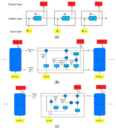
As shown in Figure 6, recurrent types mainly include the Recurrent Neural Network (RNN), Long Short-Term Memory [64] (LSTM), and Gated Recurrent Unit [65] (GRU). Gradient explosion or disappearance occurs in recurrent neural networks as parameters are increased; then, the creation of LSTM alleviates the problem of gradient explosion in the recurrent neural network, followed by GRU with fewer parameters than LSTM. At present, the LSTM is the most used network of recurrent neural networks in the lithium battery SOC estimation problem, followed by the GRU, and the recurrent neural network is not used directly [66]. The benefit of a recurrent neural network is that it can utilize the previous output as the next input, thus exploiting the relationship of the input variables; but, owing to its one-way operation and historical data calculation, it takes longer to train than neural networks that can run in parallel.

Figure 6. Recurrent Type: (a) Recurrent neural network; (b) Long short-term memory neural network; (c) Gated recurrent unit.

Ephrem et al. [67] adopted LSTM to train the lithium battery SOC model under fixed and varying ambient temperatures in the dataset [46]. In the fixed ambient temperature SOC model, the training dataset included the data under eight mixed drive cycles, and the two discharge test cases were used as the validation dataset; the test dataset was the charging test case; in the varying ambient temperature SOC model, the training dataset with 27 drive cycles included three sets of nine drive cycles recorded at 0 °C, 10 °C, and 25 °C. The test dataset included the data of another mixed-drive cycle. Both models’ input variables are voltage, current, and temperature. After evaluation, the model achieved the lowest MAE of 0.573% at 10 °C and an MAE of 1.606% with ambient temperature from 10 to 25 °C. Cui et al. [68] used LSTM with an encoder–decoder [69] structure in the dataset [43]; the input was “I_t, V_t, I_avg, V_avg”, and the test result was an RMSE of 0.56% and MAE of 0.46% in US06, which was higher than that using only LSTM and GRU in that paper. Wong et al. [70] used the undisclosed ‘UNIBO Power-tools Dataset’ as a training dataset and dataset [51] as a test dataset in the LSTM structure; the input variables were current, voltage, and temperature, and the MAE was 1.17% at 25 °C. Du et al. [71] tested two LR1865SK Li-ion battery cells at room temperature and used the dataset in [45] as the comparative case to test the model trained by LSTM; the input variables were current, voltage, temperature, cycles, energy, power, and time; the MAE was 0.872% at an average level. YANG et al. [72] used the LSTM to build a model for lithium battery SOC estimation; the data were obtained from the A123 18560 lithium battery under three drive cycles, i.e., DST, US06, and FUDS; the input vectors were current, voltage, and temperature. In addition, the model robustness was tested in the unknown initial state of the lithium battery, with the Unscented Kalman Filter [73] (UKF) method for comparison; the test results showed that the RMS of LSTM was significantly smaller than that of UKF.

1.4. Recurrent Type—GRU

YANG et al. [74] trained the model by using GRU, and the dataset was tested using three LiNiMnCoO2 batteries with DST and FUDS drive cycles; the input vectors were the current, voltage, and temperature. Then, the trained model was tested in a dataset of another material; it obtained 3.5% of max. RMS. The authors of studies [75,76,77] all used GRU as the neural network for model training; the dataset was the INR 18650-20R and A123 18650 lithium battery from the CALCE dataset [46] with inputs of voltage, current, and temperature, and the RMS error obtained from the test dataset was not significantly different. Kuo et al. [78] tested a 18650 Li-ion battery cell and used GRU with an encoder–decoder structure, in which the input vectors were current, voltage, and temperature; further, they compared this with LSTM, GRU, and a sequence-to-sequence structure, and the result showed that the MAE of their proposed neural network was lower than that of other methods at three different drive cycles and temperatures.

2. Hybrid Structure

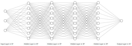
The main idea of the hybrid neural network in the estimation of the SOC of a lithium battery is to improve the prediction accuracy of the model by combining the advantages of various types of neural networks. The current common architecture in the lithium battery SOC estimation problem is a 1D-CNN as a feature extraction layer to extract deeper features of the input data, and a recurrent neural network (LSTM or GRU is used more often) as a model building layer to construct a model between the SOC and the input variables. Some scholars also added the fully connected layer (FC) before the final output layer to improve the accuracy of the model. The architecture of 1D-CNN + X + Y in lithium battery SOC estimation is depicted in Figure 7.

Figure 7. 1D-CNN + X + Y architecture diagram.

2.1. 1D-CNN + LSTM

SONG et al. [79] used a neural network combination of “1D-CNN + LSTM” to build a model with inputs of voltage, current, temperature, average voltage, and average current, for the dataset, and the 1.1 Ah A123 18650 lithium battery was tested at seven different temperatures with drive cycles of US06, FUDS. The results showed that the error of the “1D-CNN + LSTM” method was significantly smaller than that of the method that only used one neural network when tested in the test dataset and compared with the 1D-CNN and LSTM methods.

2.2. 1D-CNN + GRU + FC

HUANG et al. [80] used a “1D-CNN + GRU + FC” neural network architecture with inputs of voltage, current, and temperature; the dataset was obtained from the BAK 18650 lithium battery at seven different temperatures with drive cycles of DST and FUDS. Compared with the method of one neural network such as RNN, GRU, and a support vector machine, it achieved the lowest RMS.

2.3. NN + Filter Algorithm

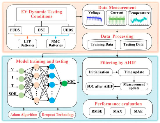
The NN + filter algorithm type uses a neural network and filter algorithm for improving Li-ion SOC estimation performance, Figure 8 is a case of that structure, which is the combination of LSTM and the adaptive H-infinity filter that can be found in [81] in more detail.

YANG et al. [82] tried to combine the advantages of both LSTM and UKF. They used LSTM and an offline training neural network to obtain a pre-trained model with the data obtained; then, the real-time data obtained were inputted into UKF and the pre-trained model, whose data input occurred after normalization. The UKF filters out the noise and improves the model performance. After this, combinations of LSTM and filtering class algorithms appear as “LSTM + CKF (Cubature Kalman Filter)” [83], “LSTM + EKF (Extended Kalman Filter)” [84], and “LSTM + AHIF (Adaptive H-infinity Filter) [81], through the test dataset, and their model performance was better than the models only trained by LSTM.

3. Trans Structure

Trans structure is mainly used to transfer the knowledge of source data to target data and in this chapter includes the section on transfer learning and transformers.

3.1. Transfer Learning

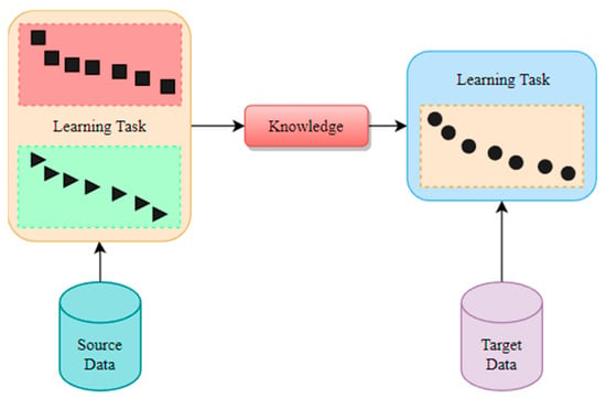
As depicted in Figure 9, the knowledge is utilized from the learning task trained by source data and that of the target data, which can improve the robustness of the model to achieve higher performance. Some researchers applied transfer learning to enhance the performance of SOC estimation.

Figure 9. Schematic of transfer learning.

Bian et al. [85] added a fully connected layer after bidirectional LSTM on this basis with inputs of voltage, current, and temperature; the datasets were three different lithium battery datasets, A123 18650, INR 18650-20R from the CALCE dataset [46] as the target dataset, and the Panasonic lithium battery dataset [49] as the pre-trained dataset. Then, they used transfer learning to transfer features from the model trained with the pre-trained dataset to the model trained with the target dataset. Compared with the method of one neural network such as RNN, LSTM, and GRU, the model of the transfer learning method achieved the lowest RMS.

Liu et al. [86] applied TCN to two different types of lithium battery data and migrated the trained model for lithium battery SOC estimation as a pre-trained model to another battery dataset by transfer learning [87]. The training dataset of the pre-trained model was “US06, HWFET, UDDS, LA92, Cycle NN”, corresponding to 25 °C, 10 °C, and 0 °C in the dataset [49], and the test set was “Cycle 1–Cycle 4”; the input vectors were current, voltage, and temperature. The model trained under 25 °C was migrated to the new lithium battery SOC model as a pre-trained model by transfer learning, the training dataset of the new lithium battery SOC model included the data measured under two mixed driving cycles in the dataset [50], the test dataset was “US06, HWFET, UDDS, LA92” in the dataset [50], and its RMS range was 0.36–1.02%.

3.2. Transformer

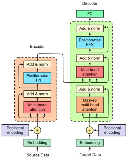
Transformer [88] is based on the encoder–decoder structure and attention mechanism, which is multi-head attention. It can enhance the connection and relation of data, and hence the transformer is applied in the natural language process, image detection, and segmentation, etc. In recent years, some scholars tried to use the structure based on the transformer for SOC estimation. The diagram of the transformer is shown in Figure 10.

Figure 10. Structure of the transformer.

Hannan et al. [89] used the structure based on the encoder of the transformer [88] to estimate SOC, and the dataset was used in [51]; the input variables were current, voltage, and temperature, and compared with different methods including DNN, LSTM, GRU, and other deep learning methods, the test performance was 1.19% for RMSE and 0.65% for MAE.

Shen et al. [90] used two encoders and one decoder of the transformer, in which the input variables were the current–temperature and voltage–temperature sequences; the dataset was obtained from [46], in which the ‘DST’ and ‘FUDS’ were used as the training dataset, and the ‘US06′ was used as test dataset. Further, they added a closed loop to improve the performance of SOC estimation; then, compared with LSTM and LSTM + UKF, the test results showed that the RMSE of their proposed method was lower than that of other methods.

This entry is adapted from the peer-reviewed paper 10.3390/machines10100912

© Text is available under the terms and conditions of the Creative Commons Attribution (CC BY) license; additional terms may apply. By using this site, you agree to the Terms and Conditions and Privacy Policy.