Stroke is a medical disease that affects millions of people worldwide per year, which leads to permanent disabilities or even death. It occurs when the regular flow of rich-oxygen blood through a brain vessel is interrupted due to a clot or a burst of it, triggering the death of brain cells and requiring prompt diagnosis and intervention after its onset to improve the prognosis significantly. The two main types of stroke are hemorrhagic and ischemic ones.
- microwave imaging
- brain stroke
- monitoring
- antenna array
1. Introduction
Stroke is a medical disease that affects millions of people worldwide per year, which leads to permanent disabilities or even death [1]. It occurs when the regular flow of rich-oxygen blood through a brain vessel is interrupted due to a clot or a burst of it, triggering the death of brain cells and requiring prompt diagnosis and intervention after its onset to improve the prognosis significantly. The two main types of stroke are hemorrhagic and ischemic ones. Because their treatment's clinical nature is the opposite, currently, the physicians support the diagnosis with well-established imaging-based techniques such as X-ray-based computerized tomography(CT) and magnetic resonance imaging(MRI). Though these technologies present high resolution and accuracy, they still have drawbacks in continuous post-acute monitoring and bedside or ambulance examinations.
Then, considering the mentioned limitations of the current systems, different new diagnosis techniques are being explored, within which is microwave imaging (MWI). It is an emerging complementary technology that maps the anatomical region of interest, i.e. the head, basing on the contrast of the electric permittivity and conductivity that exhibits healthy human tissues and pathological status under microwaves. MWI addresses some of the current issues as prehospital imaging-based diagnosis and bedside follow-up in the post-acute stage while it is cost-effective.
2. Description
In general, an MWI system consists of a set of antennas immersed in a coupling medium that works either as transmitter or receivers. These radiate an object of interest and get back its scatter response, which is used for the imaging algorithm to recover the situation. In the following, we consider and take as an example an MWI system operating around 1 GHz, and with a coupling medium with relative permittivity about 20, which are obtained from theoretical formulations and experimentally validated [2] and [3](Chapter 2). The system uses a 24-element array placed conformal to a 3D anthropomorphic phantom that mimics an average head, set up that provides adequate performance with low complexity. Meanwhile, the imaging algorithm considers a differential approach, meaning this takes as input the difference of the scattering matrix of the antennas of two different instants. This approach lets the algorithm follow the growing or shrink of the stroke. Moreover, it uses the Born Approximation to linearizer the problem considering that the variation between scenarios is focused on a small portion of the domain of interest.
3. Experimental Testing
The previously described MWI system was validated using a simplified setup with a 3D single-cavity anthropomorphic head phantom in which a 1.25 cm-radius plastic sphere was inserted, as shown in the figure below
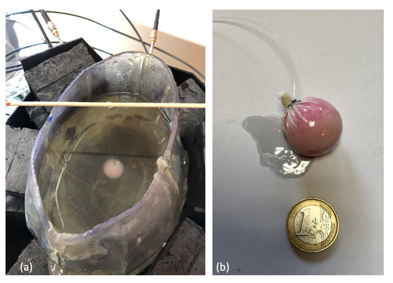
Figure. (a) Experimental set-up; (b) 1.25 cm-radius plastic sphere.
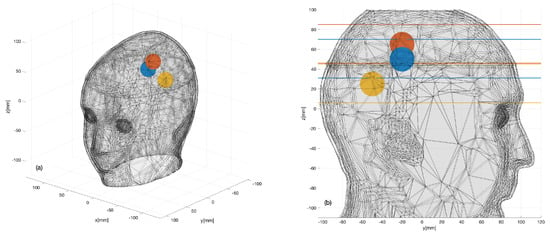
Figure. Three sphere locations (color dots) considered within the 3D head phantom: (a) 3D view; (b) 2D sagittal view.
The aim of these experiments was to identify the 3D shape and location of the sphere that was supposed to represent the region of the brain affected by the stroke. In this respect, it is important to remark that, while the plastic sphere adopted here for the sake of simplicity was not intended to mimic a hemorrhage or a clot, it showed a dielectric contrast with brain tissues which was comparable to hemorrhage but with the opposite sign. Thus, the experiment was expected to provide a meaningful, though initial, validation of the imaging capabilities of the prototype device.
A numerical assessment was performed before the experimental implementation, in both plastic and blood targets, in order to confirm the functioning of the system with a realistic scenario but with the control provided by computerized simulations (More information in the paper [3]).
To perform the experimental validation of the system, for each sphere location, two measurement sets were taken at different times. The first data-set was measured in the absence of the sphere, and the second one was taken when the sphere was positioned inside the phantom. Each pair of measured 24×24 scattering matrices were then differentiated and given as an input to the TSVD algorithm. The kernel simulated with the digital twin was exploited to generate the images, and the data processing time needed by the TSVD algorithm was negligible (less than 1 s).
The figure below shows a summary of the experimental data. The first row is the acquired data (24x24 scattering matrix), while the other rows depict the generated images and the expected position.
In all cases, the targets are very well retrieved, and the images agree with the simulation results, which confirms the expectations and the previous simulated tests.
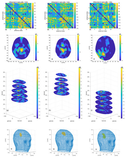
Figure. Measurement results: (a–c) differential scattering matrices; (d–f) horizontal cross-sections at sphere center and (g–i) at the various levels (the expected sphere location and shape are indicated by red circles); (j–l) the 3D rendering of the imaged stroke obtained by plotting the values of the normalized differential contrast amplitude, which are above −3 dB.
Finally reports horizontal cross-sections at various levels of the 3D reconstructed image obtained by differentiating two different sets of measurements of the same scenario (check on false positive); all the images are normalized with respect to the maximum value of the previous figure, which represents a case when the target is present.
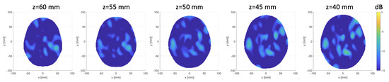
Figure. Horizontal cross-sections at various levels of the obtained 3D image, differentiating two sets of different measurements of the same scenario.
This entry is adapted from the peer-reviewed paper 10.3390/s20092607
References
- Emelia J. Benjamin; Paul Muntner; Alvaro Alonso; Marcio S. Bittencourt; Clifton W. Callaway; April P. Carson; Alanna M. Chamberlain; Alexander R. Chang; Susan Cheng; Sandeep R. Das; et al. Heart Disease and Stroke Statistics—2019 Update: A Report From the American Heart Association. Circulation 2019, 139, 56, 10.1161/cir.0000000000000659.
- Rosa Scapaticci; Loreto Di Donato; Ilaria Catapano; Lorenzo Crocco; A FEASIBILITY STUDY ON MICROWAVE IMAGING FOR BRAIN STROKE MONITORING. Progress In Electromagnetics Research B 2012, 40, 305-324, 10.2528/pierb12022006.
- Jorge Alberto Tobon Vasquez; Rosa Scapaticci; Giovanna Turvani; Gennaro Bellizzi; David Rodriguez-Duarte; Nadine Joachimowicz; Bernard Duchêne; Enrico Tedeschi; Mario R. Casu; Lorenzo Crocco; et al. A Prototype Microwave System for 3D Brain Stroke Imaging.. Sensors 2020, 20, 2607, 10.3390/s20092607.