Biaxial tensile testing is a versatile technique to address the mechanical characterization of planar materials. Typical materials tested in biaxial configuration include metal sheets, silicone elastomers, composites, thin films, textiles and biological soft tissues.
- biaxial
- tensile testing
- mechanical
1. Purposes of Biaxial Tensile Testing
A biaxial tensile test generally allows the assessment of the mechanical properties [1] and a complete characterization for uncompressible isotropic materials, which can be obtained through a fewer amount of specimens with respect to uniaxial tensile tests.[2] Biaxial tensile testing is particularly suitable for understanding the mechanical properties of biomaterials, due to their directionally oriented microstructures.[3] If the testing aims at the material characterization of the post elastic behaviour, the uniaxial results become inadequate, and a biaxial test is required in order to examine the plastic behaviour.[4] In addition to this, using uniaxial test results to predict rupture under biaxial stress states seems to be inadequate.[5][6]
Even if a biaxial tensile test is performed in a planar configuration, it may be equivalent to the stress state applied on three-dimensional geometries, such as cylinders with an inner pressure and an axial stretching.[7] The relationship between the inner pressure and the circumferential stress is given by the Mariotte formula: [math]\displaystyle{ \sigma_c = \frac{PD}{2t} }[/math] where [math]\displaystyle{ \sigma_c }[/math] is the circumferential stress, P the inner pressure, D the inner diameter and t the wall thickness of the tube.
2. Equipment
Typically, a biaxial tensile machine is equipped with motor stages, two load cells and a gripping system.
2.1. Motor Stages
Through the movement of the motor stages a certain displacement is applied on the material sample. If the motor stage is one, the displacement is the same in the two direction and only the equi-biaxial state is allowed. On the other hand, by using four independent motor stages, any load condition is allowed; this feature makes the biaxial tensile test superior to other tests that may apply a biaxial tensile state, such as the hydaulic bulge, semispherical bulge, stack compression or flat punch. [8] Using four independent motor stages allows to keep the sample centred during the whole duration of the test; this feature is particularly useful to couple an image analysis during the mechanical test. The most common way to obtain the fields of displacements and strains is the Digital Image Correlation (DIC),[8] which is a contactless technique and so very useful since it doesn't affect the mechanical results.[9]
2.2. Load Cells
Two load cells are placed along the two orthogonal load directions to measure the normal reaction forces explicated by the specimen. The dimensions of the sample have to be in accordance with the resolution and the full scale of the load cells.
A biaxial tensile test can be performed either in a load-controlled condition, or a displacement-controlled condition, in accordance with the settings of the biaxial tensile machine. In the former configuration a constant loading rate is applied and the displacements are measured, whereas in the latter configuration a constant displacement rate is applied and the forces are measured.
Dealing with elastic materials the load history is not relevant, whereas in viscoelastic materials it is not negligible. Furthermore, for this class of materials also the loading rate plays a role.[10]
2.3. Gripping System
The gripping system transfers the load from the motor stages to the specimen. Although the use of biaxial tensile testing is growing more and more, there is still a lack of robust standardized protocols concerning the gripping system. Since it plays a fundamental role in the application and distribution of the load, the gripping system has to be carefully designed in order to satisfy the Saint-Venant principle.[11] Some different gripping systems are reported below.
Clamps
The clamps are the most common used gripping system for biaxial tensile test since they allow a quite uniformly distributed load at the junction with the sample.[11] To increase the uniformity of stress in the region of the sample close to the clamps, some notches with circular tips are obtained from the arm of the sample.[12] The main problem related with the clamps is the low friction at the interface with the sample; indeed, if the friction between the inner surface of the clamps and the sample is too low, there could be a relative motion between the two systems altering the results of the test.
Sutures
Small holes are performed on the surface on the sample to connect it to the motor stages through wire with a stiffness much higher than the sample. Typically, sutures are used with square samples. In contrast to the clamps, sutures allow the rotation of the sample around the axis perpendicular to the plane; in this way they do not allow the transmission of shear stresses to the sample.[11] The load transmission is very local, thereby the load distribution is not uniform. A template is needed to apply the sutures in the same position in different samples, to have repeatability among different tests.
Rakes
This system is similar to the suture gripping system, but stiffer. The rakes transfer a limited quantity of shear stress, so they are less useful than sutures if used in presence of large shear strains. Although the load is transmitted in a discontinuous way, the load distribution is more uniform if compared to the sutures.[11]
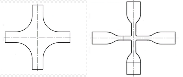
3. Specimen Shape
The success of a biaxial tensile test is strictly related to the shape of the specimen.[13] The two most used geometries are the square and cruciform shapes. Dealing with fibrous materials or fibres reinforced composites, the fibres should be aligned to the load directions for both classes of specimens, in order to minimize the shear stresses and to avoid the sample rotation.[11]
3.1. Square Samples
Square or more generally rectangular specimens are easy to obtain, and their dimension and ratio depend on the material availability. Large specimens are needed to make negligible the effects of the gripping system in the core of the sample. However this solution is very material consuming so small specimen are required. Since the gripping system is very close to the core of the specimen the strain distribution is not homogeneous.[14] [15]
3.2. Cruciform Samples
A proper cruciform sample should fulfil the following requirements:[16][17]
- maximization of the biaxially loaded area in the centre of the sample, where the strain field is uniform;
- minimization of the shear strain in the centre of the sample;
- minimization of regions of stress concentration, even outside the area of interest;
- failure in the biaxially loaded area;
- repeatable results.
Is important to note that on this kind of sample, the stretch is larger in the outer region than in the centre, where the strain is uniform.[12]
4. Method
Uniaxial stress test is typically used to measure mechanical properties of materials, while many materials exhibit various behavior when different loading stress are exerted. Thus, biaxial tensile test become one of the prospective measurements. Small Punch Test (SPT) and Hydraulic Bulge Test (HBT) are two methods applying biaxial tensile state.
4.1. Small Punch Test (SPT)
The Small Punch Test (SPT) was first developed in the 1980s as minimal invasive in-situ technique to investigate the local degradation and embrittlement of nuclear material. The SPT is a kind of miniaturized test method that only small volume specimen is required.[18] Using small volumes would not severely affect and damage an in-service component which make SPT a good method to determine the mechanical properties of unirradiated and irradiated materials or analyze small regions of structural components. [19]
In terms of the testing, the disc shaped specimen is clamped between two dies. The punch is then pushed with a constant displacement rate through the specimen. A flat punch or concave tip pushing a ball are typically used in the test.[20] After the testing, some characteristic parameters such as force-displacement curves are used to estimate yield strength, ultimate tensile stress. Considering the curves with various temperatures from SPT tensile/fracture data, ductile to brittle transition temperature (DBTT) can be calculated.[21] One thing to be noticed is that the specimen used in SPT is suggested to be very flat to reduce the stress error caused by undefined contact situation.
4.2. Hydraulic Bulge Test (HBT)
Hydraulic Bulge Test (HBT) is a method of biaxial tensile testing. It used to determine the mechanical properties such as Young’s moduli, yield strength, ultimate tensile strength, and strain-hardening properties of sheet material like thin films. HBT can better describe the plastic properties of a sheet at large strains since the strain in press forming are normally larger than the uniform strain.[22] However, the geometries of forming part are not symmetry, therefore, the true stress and strain measured by HBT will be higher than that measured by tensile test.[23]
In HBT, rupture discs and high-pressure hydraulic oil are used to cause specimen deformation which also used to avoid influence factors such as friction during small punch test. While there are constraints in test conditions, the temperature is limited by solidification and vaporization of hydraulic oil. High temperature would lead to loading failure, while low temperature result in the failure of the seal part and the leaking vapor might be dangerous.[24]
In HBT, a circular sample is normally stripped from a substrate on which they have been prepared and clamped over a hole around its periphery at the end of a cylinder. It experiences pressure from one side using hydraulic oil and then bulges and expands into a cavity with increasing pressure. The flow stress is calculated from the dome height of the bulging blank and the pressure and height can also be determined. Strain will be measured by Digital Image Correlation (DIC).[25] With the specimen thickness and clamper size being considered, the true stress and strain can be calculated.[23]
5. Analytical Solution
A biaxial tensile state can be derived starting from the most general constitutive law for isotropic materials in large strains regime: [math]\displaystyle{ \mathbf{S} = 2 \left(W_1\mathbf{I} + W_2 \left(I_1^C\mathbf{I}-\mathbf{C}\right) + W_3I_3^C \mathbf{C}^{-1}\right) }[/math] where S is the second Piola-Kirchhoff stress tensor, I the identity matrix, C the right Cauchy-Green tensor, and [math]\displaystyle{ W_1 = \frac{\partial W_0}{\partial I_1^C} }[/math], [math]\displaystyle{ W_2 = \frac{\partial W_0}{\partial I_2^C} }[/math] and [math]\displaystyle{ W_3 = \frac{\partial W_0}{\partial I_3^C} }[/math] the derivatives of the strain energy function per unit of volume in the undeformed configuration [math]\displaystyle{ W_0 }[/math] with respect to the three invariants of C.
For an uncompressible material, the previous equation becomes: [math]\displaystyle{ \mathbf{S} = 2 \left(W_1\mathbf{I} + W_2 \left(I_1^C\mathbf{I}-\mathbf{C}\right)\right) - p\mathbf{C}^{-1} }[/math] where p is of hydrostatic nature and plays the role of a Lagrange multiplier. It is worth nothing that p is not the hydrostatic pressure and must be determined independently of constitutive model of the material.
A well-posed problem requires specifying [math]\displaystyle{ S_{33} }[/math]; for a biaxial state of a membrane [math]\displaystyle{ S_{33}=0 }[/math], thereby the p term can be obtained [math]\displaystyle{ p = 2 C_{33} \left(W_1 + W_2 \left(I_1^C-C_{33}\right)\right) }[/math] where [math]\displaystyle{ C_{33} }[/math] is the third component of the diagonal of C.
According to the definition, the three non zero components of the deformation gradient tensor F are [math]\displaystyle{ F_{11} = \lambda_{11} }[/math], [math]\displaystyle{ F_{22}=\lambda_{22} }[/math] and [math]\displaystyle{ F_{33} = \frac{1}{\lambda_{11}\lambda_{22}} }[/math].
Consequently, the components of C can be calculated with the formula [math]\displaystyle{ \mathbf{C}=\mathbf{F}^T\mathbf{F} }[/math], and they are [math]\displaystyle{ C_{11} = \lambda_{11}^2 }[/math], [math]\displaystyle{ C_{22}=\lambda_{22}^2 }[/math] and [math]\displaystyle{ C_{33}=\frac{1}{\lambda_{11}^2\lambda_{22}^2} }[/math].
According with this stress state, the two non zero components of the second Piola-Kirchhoff stress tensor are: [math]\displaystyle{ S_{11} = 2 W_1\left(1-\frac{1}{\lambda_{11}^4 \lambda_{22}^2}\right)+2 W_2\left(\lambda_{22}^2-\frac{1}{\lambda_{11}^4}\right) }[/math] [math]\displaystyle{ S_{22} = 2 W_1 \left(1-\frac{1}{\lambda_{11}^2\lambda_{22}^4}\right) + 2 W_2 \left(\lambda_{11}^2-\frac{1}{\lambda_{22}^4}\right) }[/math]
By using the relationship between the second Piola-Kirchhoff and the Cauchy stress tensor, [math]\displaystyle{ \sigma_{11} }[/math] and [math]\displaystyle{ \sigma_{22} }[/math] can be calculated: [math]\displaystyle{ \sigma_{11} = 2 W_1 \left(\lambda_{11}^2-\frac{1}{\lambda_{11}^2\lambda_{22}^2}\right) + 2 W_2 \left(\lambda_{11}^2\lambda_{22}^2-\frac{1}{\lambda_{11}^2}\right) }[/math] [math]\displaystyle{ \sigma_{22} = 2 W_1 \left(\lambda_{22}^2-\frac{1}{\lambda_{11}^2\lambda_{22}^2}\right) + 2 W_2 \left(\lambda_{11}^2\lambda_{22}^2-\frac{1}{\lambda_{22}^2}\right) }[/math]
5.1. Equi-Biaxial Configuration
The simplest biaxial configuration is the equi-biaxial configuration, where each of the two direction of load are subjected to the same stretch at the same rate. In an uncompressible isotropic material under a biaxial stress state, the non zero components of the deformation gradient tensor F are [math]\displaystyle{ F_{11}=F_{22}=\lambda }[/math] and [math]\displaystyle{ F_{33}=\frac{1}{\lambda^2} }[/math].
According to the definition of C, its non zero components are [math]\displaystyle{ C_{11}=C_{22}=\lambda^2 }[/math] and [math]\displaystyle{ C_{33}=\frac{1}{\lambda^4} }[/math]. [math]\displaystyle{ S_{11} = S_{22} = 2 W_1 \left(1-\frac{1}{\lambda^6}\right) + 2 W_2 \left(\lambda^2 - \frac{1}{\lambda^4}\right) }[/math]
The Cauchy stress in the two directions is: [math]\displaystyle{ \sigma_{11} = \sigma_{22} = 2 W_1 \left(\lambda^2-\frac{1}{\lambda^4}\right) + 2 W_2 \left(\lambda^4-\frac{1}{\lambda^2}\right) }[/math]
5.2. Strip Biaxial Configuration
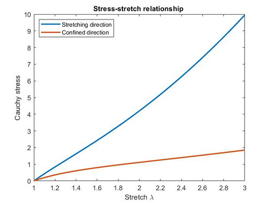
A strip biaxial test is a test configuration where the stretch of one direction is confined, namely there is a zero displacement applied on that direction. The components of the C tensor become [math]\displaystyle{ C_{11}=\lambda^2 }[/math], [math]\displaystyle{ C_{22}=1 }[/math] and [math]\displaystyle{ C_{33}=\frac{1}{\lambda^2} }[/math]. It is worth nothing that even if there is no displacement along the direction 2, the stress is different from zero and it is dependent on the stretch applied on the orthogonal direction, as stated in the following equations: [math]\displaystyle{ S_{11} = 2 W_1 \left(1-\frac{1}{\lambda^4}\right) + 2 W_2\left(1-\frac{1}{\lambda^4}\right) }[/math] [math]\displaystyle{ S_{22} = 2 W_1 \left(1-\frac{1}{\lambda^2}\right) + 2 W_2 \left(\lambda^2-1\right) }[/math]
The Cauchy stress in the two directions is: [math]\displaystyle{ \sigma_{11} = 2 W_1 \left(\lambda^2-\frac{1}{\lambda^2}\right)+2W_2\left(\lambda^2-\frac{1}{\lambda^2}\right) }[/math] [math]\displaystyle{ \sigma_{22} = 2 W_1 \left(\lambda^2-1\right) + 2 W_2 \left(\lambda^4-\lambda^2\right) }[/math]
The strip biaxial test has been used in different applications, such as the prediction of the behaviour of orthotropic materials under a uniaxial tensile stress,[26] delamination problems,[27] and failure analysis.[28]
6. FEM Analysis
Finite Element Methods (FEM) are sometimes used to obtain the material parameters.[29][30][31] The procedure consists of reproducing the experimental test and obtain the same stress-stretch behaviour; to do so, an iterative procedure is needed to calibrate the constitutive parameters. This kind of approach has been demonstrated to be effective to obtain the stress-stretch relationship for a wide class of hyperelastic material models (Ogden, Neo-Hooke, Yeoh, and Mooney-Rivlin).[12]
7. Standards
- ISO 16842:2014 metallic materials – sheet and strip – biaxial tensile testing method using a cruciform test piece.
- ISO 16808:2014 metallic materials – sheet and strip – determination of biaxial stress-strain curve by means of bulge test with optical measuring systems.
- ASTM D5617 – 04(2015) – Standard Test Method for Multi-Axial Tension Test for Geosynthetics.
- DIN EN 17117 – A German standard describes methods of the test using biaxial stress states for the determination of the ten-sile stiffness properties of biaxially oriented coated fabrics
The content is sourced from: https://handwiki.org/wiki/Engineering:Biaxial_tensile_testing
References
- Uhlemann, Jörg; Stranghöner, Natalie (2016). "Refined Biaxial Test Procedures for the Determination of Design Elastic Constants of Architectural Fabrics". Procedia Engineering 155: 211–219. doi:10.1016/j.proeng.2016.08.022. https://dx.doi.org/10.1016%2Fj.proeng.2016.08.022
- Redaelli, A. (2007). Biomeccanica : analisi multiscala di tessuti biologici. Bologna: Pàtron. ISBN 978-8855531764.
- Holzapfel, Gerhard A.; Ogden, Ray W. (July 2009). "On planar biaxial tests for anisotropic nonlinearly elastic solids. A continuum mechanical framework". Mathematics and Mechanics of Solids 14 (5): 474–489. doi:10.1177/1081286507084411. https://dx.doi.org/10.1177%2F1081286507084411
- Beccarelli, Paolo (2015). Biaxial Testing for Fabrics and Foils. SpringerBriefs in Applied Sciences and Technology. doi:10.1007/978-3-319-02228-4. ISBN 978-3-319-02227-7. https://dx.doi.org/10.1007%2F978-3-319-02228-4
- Soden, P.D.; Hinton, M.J.; Kaddour, A.S. (September 2002). "Biaxial test results for strength and deformation of a range of E-glass and carbon fibre reinforced composite laminates: failure exercise benchmark data". Composites Science and Technology 62 (12–13): 1489–1514. doi:10.1016/S0266-3538(02)00093-3. https://dx.doi.org/10.1016%2FS0266-3538%2802%2900093-3
- Welsh, J.S.; Adams, D.F. (September 2000). "Development of an electromechanical triaxial test facility for composite materials". Experimental Mechanics 40 (3): 312–320. doi:10.1007/BF02327505. https://dx.doi.org/10.1007%2FBF02327505
- Hartmann, Stefan; Gilbert, Rose Rogin; Sguazzo, Carmen (April 2018). "Basic studies in biaxial tensile tests: Biaxial tensile experiments". GAMM-Mitteilungen 41 (1): e201800004. doi:10.1002/gamm.201800004. https://dx.doi.org/10.1002%2Fgamm.201800004
- Seymen, Y.; Güler, B.; Efe, M. (November 2016). "Large Strain and Small-Scale Biaxial Testing of Sheet Metals". Experimental Mechanics 56 (9): 1519–1530. doi:10.1007/s11340-016-0185-7. https://dx.doi.org/10.1007%2Fs11340-016-0185-7
- McCormick, Nick; Lord, Jerry (December 2010). "Digital Image Correlation". Materials Today 13 (12): 52–54. doi:10.1016/S1369-7021(10)70235-2. https://dx.doi.org/10.1016%2FS1369-7021%2810%2970235-2
- Guo, Hui; Chen, Yu; Tao, Junlin; Jia, Bin; Li, Dan; Zhai, Yue (September 2019). "A viscoelastic constitutive relation for the rate-dependent mechanical behavior of rubber-like elastomers based on thermodynamic theory". Materials & Design 178: 107876. doi:10.1016/j.matdes.2019.107876. https://dx.doi.org/10.1016%2Fj.matdes.2019.107876
- Fehervary, Heleen; Vastmans, Julie; Vander Sloten, Jos; Famaey, Nele (December 2018). "How important is sample alignment in planar biaxial testing of anisotropic soft biological tissues? A finite element study". Journal of the Mechanical Behavior of Biomedical Materials 88: 201–216. doi:10.1016/j.jmbbm.2018.06.024. PMID 30179794. https://lirias.kuleuven.be/handle/123456789/630198.
- Fujikawa, M.; Maeda, N.; Yamabe, J.; Kodama, Y.; Koishi, M. (November 2014). "Determining Stress–Strain in Rubber with In-Plane Biaxial Tensile Tester". Experimental Mechanics 54 (9): 1639–1649. doi:10.1007/s11340-014-9942-7. https://dx.doi.org/10.1007%2Fs11340-014-9942-7
- Makris, A.; Vandenbergh, T.; Ramault, C.; Van Hemelrijck, D.; Lamkanfi, E.; Van Paepegem, W. (April 2010). "Shape optimisation of a biaxially loaded cruciform specimen". Polymer Testing 29 (2): 216–223. doi:10.1016/j.polymertesting.2009.11.004. https://dx.doi.org/10.1016%2Fj.polymertesting.2009.11.004
- Thom, Holger (August 1998). "A review of the biaxial strength of fibre-reinforced plastics". Composites Part A: Applied Science and Manufacturing 29 (8): 869–886. doi:10.1016/S1359-835X(97)00090-0. https://dx.doi.org/10.1016%2FS1359-835X%2897%2900090-0
- Gdoutos, Emmanuel (2002). Recent advances in experimental mechanics: in honor of Isaac M. Daniel. Dordrecht: Kluwer Academic Publishers. ISBN 1-4020-0683-7.
- Tobajas, Rafael; Elduque, Daniel; Ibarz, Elena; Javierre, Carlos; Gracia, Luis (2020-05-23). "A New Multiparameter Model for Multiaxial Fatigue Life Prediction of Rubber Materials". Polymers 12 (5): 1194. doi:10.3390/polym12051194. PMID 32456238. http://www.pubmedcentral.nih.gov/articlerender.fcgi?tool=pmcentrez&artid=7285379
- Geiger, M.; Hußnätter, W.; Merklein, M. (August 2005). "Specimen for a novel concept of the biaxial tension test". Journal of Materials Processing Technology 167 (2–3): 177–183. doi:10.1016/j.jmatprotec.2005.05.028. https://dx.doi.org/10.1016%2Fj.jmatprotec.2005.05.028
- Rasche, Stefan; Strobl, Stefan; Kuna, Meinhard; Bermejo, Raul; Lube, Tanja (2014-01-01). "Determination of Strength and Fracture Toughness of Small Ceramic Discs Using the Small Punch Test and the Ball-on-three-balls Test" (in en). Procedia Materials Science. 20th European Conference on Fracture 3: 961–966. doi:10.1016/j.mspro.2014.06.156. ISSN 2211-8128. https://www.sciencedirect.com/science/article/pii/S2211812814001576.
- Pullin, Rhys; Jenkins, Ifan; Cernescu, Anghel; Edwards, Allen (2020-07-30). "Equivalent biaxial strain evaluation in small punch testing using acoustic emission". The Journal of Strain Analysis for Engineering Design 56 (3): 173–180. doi:10.1177/0309324720944067. ISSN 0309-3247. http://dx.doi.org/10.1177/0309324720944067.
- Bruchhausen, M.; Holmström, S.; Simonovski, I.; Austin, T.; Lapetite, J. -M.; Ripplinger, S.; de Haan, F. (2016-12-01). "Recent developments in small punch testing: Tensile properties and DBTT" (in en). Theoretical and Applied Fracture Mechanics. Small Scale Testing in Fracture Mechanics 86: 2–10. doi:10.1016/j.tafmec.2016.09.012. ISSN 0167-8442. https://www.sciencedirect.com/science/article/pii/S0167844216301677.
- "Small Punch Test - Helmholtz-Zentrum Dresden-Rossendorf, HZDR" (in de). https://www.hzdr.de/db/Cms?pOid=13993&pNid=2708.
- Ranta-Eskola, A. J. (1979-01-01). "Use of the hydraulic bulge test in biaxial tensile testing" (in en). International Journal of Mechanical Sciences 21 (8): 457–465. doi:10.1016/0020-7403(79)90008-0. ISSN 0020-7403. https://dx.doi.org/10.1016/0020-7403%2879%2990008-0.
- Dimarn, Autthasit; Thanadngarn, Charn; Buakaew, Vichit; Neamsup, Yongyuth (2014-06-02). Sirisoonthorn, Somnuk. ed. "Mechanical properties testing of sheet metal by hydraulic bulge test". International Conference on Experimental Mechanics 2013 and Twelfth Asian Conference on Experimental Mechanics (SPIE) 9234: 135–145. doi:10.1117/12.2054257. Bibcode: 2014SPIE.9234E..0KD. https://www.spiedigitallibrary.org/conference-proceedings-of-spie/9234/92340K/Mechanical-properties-testing-of-sheet-metal-by-hydraulic-bulge-test/10.1117/12.2054257.full.
- Wang, Hankui; Xu, Tong; Shou, Binan (2016-12-30). "Determination of Material Strengths by Hydraulic Bulge Test". Materials 10 (1): 23. doi:10.3390/ma10010023. ISSN 1996-1944. PMID 28772379. Bibcode: 2016Mate...10...23W. http://www.pubmedcentral.nih.gov/articlerender.fcgi?tool=pmcentrez&artid=5344578
- "Bulge and Dome Testing" (in en-US). 2020-11-26. https://ahssinsights.org/forming/testing-characterization-forming/bulge-and-dome-testing/.
- Komatsu, Takuya; Takatera, Masayuki; Inui, Shigeru; Shimizu, Yoshio (March 2008). "Relationship Between Uniaxial and Strip Biaxial Tensile Properties of Fabrics". Textile Research Journal 78 (3): 224–231. doi:10.1177/0040517507083439. https://dx.doi.org/10.1177%2F0040517507083439
- Liechti, K. M.; Becker, E. B.; Lin, C.; Miller, T. H. (March 1989). "A fracture analysis of cathodic delamination in rubber to metal bonds". International Journal of Fracture 39 (1–3): 217–234. doi:10.1007/BF00047451. https://dx.doi.org/10.1007%2FBF00047451
- 3.0.CO;2-1. https://dx.doi.org/10.1002%2F%28SICI%291521-4087%28199912%2924%3A6%3C349%3A%3AAID-PREP349%3E3.0.CO%3B2-1" id="ref_28">Renganathan, K.; Rao, B. Nageswara; Jana, M. K. (1999). "Failure Assessment on a Strip Biaxial Tension Specimen for a HTPB-Based Propellant Material". Propellants, Explosives, Pyrotechnics 24 (6): 349–352. doi:10.1002/(SICI)1521-4087(199912)24:6<349::AID-PREP349>3.0.CO;2-1. https://dx.doi.org/10.1002%2F%28SICI%291521-4087%28199912%2924%3A6%3C349%3A%3AAID-PREP349%3E3.0.CO%3B2-1
- Budiarsa, I. Nyoman; Subagia, I.D.G. Ary; Widhiada, I. Wayan; Suardana, Ngakan P.G. (2015). "Characterization of Material Parameters by Reverse Finite Element Modelling Based on Dual Indenters Vickers and Spherical Indentation". Procedia Manufacturing 2: 124–129. doi:10.1016/j.promfg.2015.07.022. https://dx.doi.org/10.1016%2Fj.promfg.2015.07.022
- Rojicek, J. (2010-05-17). "Identification of Material Parametres by Fem". MM Science Journal 2010 (2): 186–189. doi:10.17973/MMSJ.2010_06_201008. https://dx.doi.org/10.17973%2FMMSJ.2010_06_201008
- Tarantino, Angelo Marcello; Majorana, Carmelo; Luciano, Raimondo; Bacciocchi, Michele (2021-02-07). "Special Issue: "Advances in Structural Mechanics Modeled with FEM"". Materials 14 (4): 780. doi:10.3390/ma14040780. PMID 33562220. Bibcode: 2021Mate...14..780T. http://www.pubmedcentral.nih.gov/articlerender.fcgi?tool=pmcentrez&artid=7914604