Your browser does not fully support modern features. Please upgrade for a smoother experience.
Please note this is an old version of this entry, which may differ significantly from the current revision.
Subjects:
Engineering, Civil
Flood is one of the most destructive natural disasters, causing significant economic damage and loss of lives. Numerous methods have been introduced to estimate design floods, which include linear and non-linear techniques. Since flood generation is a non-linear process, the use of linear techniques has inherent weaknesses. To overcome these, artificial intelligence (AI)-based non-linear regional flood frequency analysis (RFFA) techniques have been introduced over the last two decades.
- regional flood frequency analysis
- artificial neural networks
- flood
- artificial intelligence
1. Introduction
Flood is one of most devastating natural disasters, resulting in significant economic losses including human deaths [1,2]. This damages both rural and urban infrastructure like bridge and drainage systems [3,4]. Flood generally leaves undesirable sediments and debris in the affected lands [5,6], which can disrupt transportation networks [7], clog drainage infrastructure and sewers [8,9] and may make lands unproductive. The cleaning up of flood debris is usually costly, not to mention the disruption to the daily lives of the community involved [10,11]. Due to climate change, the frequency and magnitude of floods are increasing [12].
Flood forecasting requires significant efforts, and it is usually the responsibility of a large government organisation. Governments spend a significant amount on various projects to identify flood-safe areas, which are used to build cities. Researchers have developed numerous methods to estimate design floods, which are used to build flood-safe infrastructure [13,14]. Design flood is defined as a flood level or discharge associated with a return period or annual exceedance probability such as a 100-year flood.
In addition to traditional techniques, like the rational method, physical and numerical [15,16] models have been proposed for design flood estimation. Most of the physical models require in-depth knowledge of flood processes [17,18], making them difficult to use in practice. Van den Honert and McAneney [19] pointed out the common limitations associated with these physical models [20,21], which include model inaccuracies resulting in systematic errors (over or underestimation of design floods) [22,23]. On the other hand, data-driven models have been quite popular for flood estimation in recent years [24]. Examples include a quantile regression technique and a probabilistic rational method [25]. This is because they usually consider climate factors and catchment characteristics in developing models, which are easier to apply [26,27]. A flood frequency analysis (FFA) is the most popular method to estimate design floods, which uses observed peak discharge data disregarding catchment characteristics [28,29]. A normal distribution [30,31], log-normal distribution [32,33], Gumbel distribution [34,35], generalised extreme value distribution and log-Pearson type III distribution [36,37] are some of the most commonly used flood frequency distributions in FFA. One of the major limitations of FFA is the lack of long and good quality recorded flood data at the location of interest. To overcome data limitations, hydrologists have proposed a regional flood frequency analysis (RFFA), which attempts to estimate design floods at an ungauged catchment based on the concept of a homogeneous region, which pools observed flood data from a group of similar catchments to estimate design floods at the ungauged catchment [38,39]. This method became more popular among researchers than physical models because it saves time and resources [40]. Probabilistic rational method (PRM) [41], multiple linear regression (MLR) [42,43], quantile regression techniques (QRT) [44,45], and index flood method (IFM) [46,47] are some of the most commonly used RFFA techniques. However, some of the early RFFA techniques (e.g., rational method) have lost their popularity due to their inconsistency and inappropriate model assumptions.
In the past two decades, scientists suggested hybrid or mixed methods to increase the relative accuracy of RFFA models [48,49]. Although some early linear models have been improved, they may not be accurate under some circumstances as flood generation is basically a non-linear process [50]. Hydrologists attempted to apply non-linear methods in RFFA such as a non-linear regression analysis (where log-transformation of the variables is considered). Artificial intelligence (AI)-based methods are also non-linear, but more powerful than simple non-linear models like log-log ones as they can consider many different combinations of variables and complex non-linear processes in model building. Given that the majority of flood estimation methods are data driven, they require a great deal of simplification and assumptions to be practical, accessible, and implementable [51,52]. They require relatively fewer input data and minimal knowledge of fundamental physical processes involved. Over the last two decades, non-linear AI-based RFFA methods have grown in popularity over physical models as these provide more accurate results and are easier to apply [53,54]. Artificial neural networks (ANNs) [55,56], support vector regression (SVR) [57,58,59,60], adaptive neuro-fuzzy inference system (ANFIS) [61,62], genetic algorithms (GA) [63,64] and hybrid, mixed and combined approaches [65,66] are some of the most popular AI-based flood estimation methods. As AI-based models are relatively new in flood estimation, it is not easy to decide which one is to be applied for a given problem [67,68].
There are several important aspects to consider when building models based on AI. Firstly, these models like all other data-driven models need enough data to develop and test the model [67]. If adequate data exist, it is often possible to build, test, and evaluate an AI-based model (similar to many other RFFA models) by dividing the data into training, test, and evaluation data sub-sets [69,70]. Cross-validation is also often used in building RFFA models when less data samples are available [71]. The more data used in the modeling, the less generalization error occurs, meaning that the final model can be used on different sites with limited or no data available. Other benefits of having adequate data include the simplicity of using different distribution methods, the ability to account for lost data or missing variables, and, most crucially, the ability to train and validate the model multiple times to develop the best possible model [72,73]. However, it should be noted that data quality is of significant importance in developing and testing accurate models.
2. AI-Based RFFA Methods
Figure 2 illustrates how to develop an AI-based RFFA model. It is important to identify input variables. Some of the most used input variables include catchment area (A), longitude (LON), latitude (LAT), elevation (EV), drainage density (DD), average annual maximum daily precipitation (AP), rainfall intensity (I), vegetation coverage (VC), slope (SL), and relative elevation (RE), fraction forested area (F), mean annual evapotranspiration (MAE), shape factor (SF), and stream density (SDEN). Output variables include maximum stream flow, flood quantiles, and time to peak. Collected data are then standardised to avoid a scaling problem. To build a reliable model, training, validation [69,70], and test data are required. Different statistical measures are used to compare alternative models such as RMSE, RMSNE, and R2.
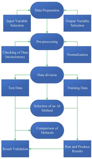
Figure 2. Steps in building an AI-based RFFA model.
2.1. ANN-Based RFFA Models
The ANN performs like a human nervous system in that it learns from previous trials and decides how to come up with a better model by exploiting the best possible links between dependent (flood quantiles such as Q10) and independent variables (such as rainfall) in a series of steps. ANN, as a data-driven tool, does not require any physical knowledge of flood processes involved [78,79]. One of the limitations of this method is lack of physical interpretation of the developed models.
Shu and Burn [51] compared the ANN with a parametric regression analysis in one of the first articles on the AI-based RFFA. They found that a properly developed ANN model outperforms both linear (REG-OLS) and non-linear (REG-NONLINEAR) regression-based methods. They also compared the results of a single ANN to those of ANN ensembles, concluding that the latter provided more accurate flood estimates. Jingyi and Hall [80] compared four different models, including the residuals method, Ward’s method, fuzzy c-mean, and a variation of the ANN, known as the Kohonen network. They found that, while other methods may be somewhat useful, the ANN method produced the lowest standard error of estimate and could be a useful method if adequate data from enough sites are available.
Dawson et al. [81] applied ANN using data from 850 stations. They compared the results of the ANN method to those of multiple regression models and found that ANN outperformed the other models. They noted that because there is little need to understand the physics of flood generation processes, scientists from all disciplines, not just hydrologists, could use the ANN method. Shu and Ouarda [56] developed RFFA models based on ANN and CCA using data from 151 catchments and found that the ANN–CCA combination provided better generalisation and accuracy. Srinivas et al. [49] used AI-based RFFA and regression methods involving various AI-based algorithms. To determine the best approach for data clustering, a regression analysis, CCA, and FCM algorithms were compared. They found that leave-one-out cross-validation based on the FCM algorithm produced better results when evaluating the accuracy of the estimated flood quantities.
2.3. SVM-Based RFFA Models
The SVM method is widely used for classification, which examines data at higher dimensions [107,108]. Several types of kernels assist SVM in classifying data by minimising data margins, eliminating outliers, and focusing on relationships between the test and training data. The most common kernel types used for developing SVM-based models include linear, polynomial, radial basis function (RBF), and sigmoid function. Among these, the SVM-based RBF kernel is the most used method that produces robust and consistent results.
Gizaw and Gan [109] developed RFFA-based ANN and SVR methods using data collected from 49 stations in Canada. When the results of these two methods were compared, they found that the SVR method outperformed the ANN in terms of consistency and generalisation ability. They also mentioned that better SVR performance could be attributed to smaller datasets, whereas ANN would most likely produce more accurate results for larger datasets. Sharifi Garmdareh et al. [110] estimated design floods using SVR, ANFIS, ANN, and NLR methods using more than 20 years of recorded data from 55 hydrometric stations in Iran. They tested various strategies for determining the best combination of input variables and found that gamma testing (GT) was the most effective, which can improve the result of ANFIS and SVR over a single method and that using GT reduced the number of input variables. They also noted that combining GT with the ANFIS produced the best results, followed by GT + SVR.
Ghaderi et al. [111] used ANFIS, SVM, and GEP to estimate flood quantiles with a 50-year return period. From 21 years of data collected from 47 catchments in Iran, they used GM and M-test to identify the most important predictor variables and the best ratio of test and training data. They compared the results of the three methods and noted that all three were “good” in terms of NASH, with the SVM method slightly outperforming the others in terms of R2 and RMSE. Vafakhah and Bozchaloei [112] used SVR, ANN, and NLR to estimate design floods using data collected from 33 stations in Iran over 20 years. They noted that, according to RRMSE and NASH, SVR is the most efficient method of the three and can be used for regional flood duration curve analysis.
Haddad and Rahman [65] used 25 to 82 years of data from 202 catchments in Australia to evaluate 15 different combinations of multidimensional scaling (MDS), bayesian generalised least squares (BGLSR), and SVR methods to estimate design floods. They found that the MDS-based SVR method with RBF kernel outperforming others, including linear, polynomial, RBF, and sigmoid kernels, in terms of consistency and accuracy of the results. They also noted that using MDS improved the overall performance of all the methods.
Allahbakhshian-Farsani et al. [59] used 19 years of data from 54 hydrometric stations in Iran to compare the performance of several AI-based RFFA methods. This study employed methods such as SVR, multivariate adaptive regression spline (MARS), boosted regression trees (BRT), and projection pursuit regression (PPR). Using various statistical indices such as NASH, RMSE, RMSE, and R2, they noted that the SVR model based on the RBF kernel outperformed all the others, including non-linear regression.
From the above discussion it can be stated that both SVM and SVR were used in RFFA. A large set of catchments are needed to group them into homogeneous sub-sets which can then be subjected to SVR to estimate flood quantiles.
2.4. GA and Hybrid Type of AI-Based RFFA Models
Hybrid models typically produce better results. As shown in Table 1, many scientists have conducted experiments based on combining various AI-based RFFA models. Some of the most common hybrid models include genetic algorithm (GA) combined with ANN or ANFIS. The GA is commonly used as a hybrid method in conjunction with other methods, particularly ANN [106]. Another popular hybridisation technique used in RFFA is the combination of canonical correlation analysis (CCA) with ANN and ANN ensembles, as well as ANFIS methods. CCA improves the performance and reduces the complexity of ANN-based RFFA models by exploiting regional flood data [92,97].
Table 1. Summary of AI-based RFFA studies (* indicates the best model) (ANN = Artificial neural network; GA = Genetic algorithm, BGLS-QRT-ROI: Bayesian generalized least squares QRT combined with region of influence approach, BNN = Backpropagation neural network, CANFIS = Co-active neuro fuzzy inference system, GEP = Gene-expression programming, GRNN = generalized regression neural networks, LGP = Linear genetic programming (LGP), LR = Linear regression, M5 = M5 model tree, MLP = Multi-layer perceptrons, MLR = Multiple linear regression, MNLR = Multiple non-linear regression, QRT = Quantile regression technique, RBNN = Radial basis function-based neural networks, G-EANN = generalized ANN-Ensembles, EANN = ANN-Ensembles, GAANN = GA-based ANN, BPANN = Back propagation for ANN, FIS = Fuzzy inference system, CCA = canonical correlation analysis, NLCCA = Non-linear canonical correlation analysis, BGLSR = Bayesian generalised least squares, MDS = multidimensional scaling, MARS = multivariate adaptive regression spline, BRT = boosted regression trees, PPR = projection pursuit regression, WNN = wavelet neural network and RFR = random forest regression).
| Reference | Author, Year | Model | Predictor Variables (Inputs) |
Model Output | Catchment, Year |
Journal | Country (Catchment) | RMSE * | RRMSE/NASH * | R2 * |
|---|---|---|---|---|---|---|---|---|---|---|
| [102] | Zalnezhad et al., 2022 | ANFIS(FCM) * ANFIS(SC) ANFIS(GP) QRT |
A, I, MAR, SF, MAE, SDEN, S1085, FOR | Q2–100 | 181 Stations 40–89 Year |
Water | Australia | 50.88 | RRMSE = 0.78 | NA |
| [97] | Desai and Ouarda, 2021 | CCA-RFR * PFR CCA-GAM EANN ANN CCA-MLR CCA-Kriging CCA-EANN CCA-ANN |
A, MBS, FAL, AMP, AMD | Q10–100 | 151 stations, ≥15 year | Journal of Hydrology | Canada (Quebec) |
0.05 | NASH = 0.57 RRMSE = 29.44 |
NA |
| [96] | Linh et al., 2021 | WNN * ANN |
SLP, SST | Max monthly discharge (MAD) | 3 stations, 37 years |
Acta Geophysica | Iran (Golestan Dam, Madarsoo) |
0.68 | NASH = 0.99 | 0.99 |
| [59] | Allahbakhshian-Farsani et al., 2020 | SVR * MARS BRT PPR NLR |
A, AA, AMP, MXP, NDP, CC, CR, TC, P, SL, DD, SS, MBS, PF, SDT, RA, BL, FLA, FOR, RLA, DA, WA, EL, MXEL, MNEL | Q2–200 | 54 stations, 19 years |
Water Resources Management | Iran (Karun and Karkhe River) |
50.70 | NASH = 0.94 RRMSE = 63.93 | 0.96 |
| [95] | Kordrostami et al., 2020 | ANN | A, AEV, AMP, FOR, I, SS, SF and DD | Q5–100 | 88 stations, 25–82 years |
Geosciences | Australia (New South Wales) |
NA | RRMSE = 0.48 | 0.74 |
| [65] | Haddad and Rahman, 2020 | MDS-SVR * MDS-BGLSR |
A, AEV, SF, DD, SS, FOR, I and AMP | Q2–100 | 202 stations, 25–82 years |
Natural Hazards | Australia (New South Wales and Victoria) |
NA | RRMSE = 56 | 0.78 |
| [112] | Vafakhah and Khosrobeigi Bozchaloei, 2020 | SVR * ANN NLR |
A, AA, AEV, P, MBS, MXEL, MNEL, EL, SL, DD, SS, AMP, T, PF, RLA, BL, GA, RA | Q2–90 | 33 Stations, 20 years | Water Resources Management | Iran (Namak Lake) |
0.11 | NASH = 0.91 RRMSE = 1.45 |
0.96 |
| [111] | Ghaderi et al., 2019 | SVM * ANFIS GEP |
A, P, MBS, EL, L, SL, SS, DD, MXSO, FF, L, CR, CC, AMP, MXP, BL, FOR | Q50 | 47 stations, 21 years |
Arabian Journal of Geosciences | Iran (South-west) |
239.94 | NASH = 0.75 | 0.76 |
| [110] | Sharifi Garmdareh et al., 2018 | ANFIS * SVR ANN NLR |
A, AEV, P, DD, MXEL, MNEL, MBS, EL, SL, SS, T, AMP, | Q2–100 | 55 stations, 20 years | Hydrological Sciences Journal | Iran (Namak Lake) |
8.40 | NASH = 0.90 | 0.95 |
| [67] | Aziz et al., 2017 | ANN * GEP * QRT |
A, AEV, AMP, SS, I | Q2–100 | 452 stations, 25–75 years | Stochastic Environmental Research and Risk Assessment | Australia (New South Wales, Victoria, Queensland and Tasmania) |
Na | NASH for ANN for smaller ARIs = 0.78 NASH for GEP for larger ARIs = 0.73 |
NA |
| [92] | Ouali et al., 2017 | NLCCA-GAM * NLCCA-EANN CCA-ANN CCA-EANN NLCCA-ANN NLCCA-GAM/ STPW |
A, MBS, FAL, AMP, AMD | Q10–100 | 151, 204 and 69 stations, ≥15 years | Journal of Advances in Modeling Earth Systems | Canada and United states (Quebec, Arkansas, Texas) |
NA | RRMSE = 0.28 NASH > 0.8 |
NA |
| [109] | Gizaw and Gan, 2016 | SVR * ANN |
A, SS, SL, TC, I, AMP | Q10–100 | 26 and 23 stations, ≥15 years |
Journal of Hydrology | Canada (British Columbia, Ontario) |
46.2 | NA | 0.7 |
| [106] | Aziz et al., 2016 | ANN * GAANN CANFIS GEP |
A, AEV, I, AMP, SS, | Q2–100 | 452 Stations, 25–75 years |
Artificial Neural Network Modelling (Book) | Australia (New South Wales, Victoria, Queensland and Tasmania) |
NA | NASH = 0.69 | NA |
| [61] | Kumar et al., 2015 | FIS * ANN L-moments (PE3) |
A, AMP, SDT, EL | Q2–1000 | 17 stations, 15–29 years | Water Resources Management | India (Godavari river) |
2.32 | Na | NA |
| [114] | Aziz et al., 2015 | GAANN BPANN |
A, I | Q2–100 | 452 stations, 25–75 years | Natural Hazards | Australia (New South Wales, Victoria, Queensland, and Tasmania) |
NA | NA | NA |
| [105] | Bozchaloei and Vafakhah, 2015 | ANFIS * ANN NLR |
A, AA, AEV, P, MBS, MXEL, MNEL, EL, SL, DD, SS, AMP, T, PF, RLA, BL, GA, RA | Q2–92 | 33 stations, 20 years | Journal of Hydrologic Engineering | Iran (Namak Lake) |
0.008 | NASH = 0.92 | 0.99 |
| [87] | Durocher et al., 2015 | PPR * | A, SL, SS, MBS, FOR, FAL, AMP, AMPS, AMPL, MLS, AMD | Q10–100 | 151 stations, ≥15 years | Journal of Hydrometeorology | Canada (Quebec) |
NA | RRMSE = 0.40 | NA |
| [86] | Alobaidi et al., 2015 | G-EANN * EANN |
A, MBS, FAL, AMD, AMP | Q10–100 | 151 stations, ≥15 years | Advances in Water Resources | Canada (Quebec) |
NA | RRMSE = 0.34 | NA |
| [85] | Aziz et al., 2014 | ANN * QRT |
A, AEV, AMP, SS, I | Q2–100 | 452 stations, 25–75 years | Stochastic Environmental Research and Risk Assessment | Australia (New South Wales, Victoria, Queensland, Tasmania) |
NA | NA | NA |
| [103] | Aziz et al., 2013 | BGLS-QRT-ROI * CANFIS | A and I | Q2–100 | 452 stations, 25–75 years |
Journal of Hydrological Environment Resources | Australia (New South Wales, Victoria, Queensland, and Tasmania) |
NA | NA | NA |
| [84] | Seckin et al., 2013 | MLP * L-moment RBNN GRNN MLR MNLR |
A, EL, LAT, LON, and RP | Q1.111–1000 | 13 stations, 10-39 years | Water Resources Management | Turkey (East Mediterranean River) |
0.173 | NA | 0.84 |
| [113] | Seckin and Guven, 2012 | GEP * LGP LR |
A, EL, LAT, LON, and RP | Q25.7–174.3 | 543 stations, ≥15 years |
Water Resource Management | Turkey (Rivers across the country) |
NA | NA | 0.57 |
| [83] | Singh et al., 2010 | BNN * M5 |
A, MRD, AMP, RP, MBS and FOR | Q2.33 | 93 stations, 10–83 years | Water Resources Management | India (Catchments across the country) |
NA | NA | NA |
| [82] | Ouarda and Shu, 2009 | ANN * Multiple regression model |
A, FAL, FOR, AMD, AMPL, NT27, CN | Q2–10 | 134 stations, ≥10 years | Water Resources Research | Canada (Quebec) |
27.33 | NASH = 0.96, RRMSE = 36.17 | NA |
| [55] | Shu and Ouarda, 2008 | ANFIS * ANN NLR NLR-R |
A, MBS, FAL, AMP, AMD, HDB, TOPO | Q10–100 | 151 stations- ≥15 years | Journal of Hydrology | Canada (Quebec) | 316 | NASH = 0.85 RRMSE = 57 |
NA |
| [49] | Srinivas et al., 2008 | SOFM * CCA Regional regression |
A, SS, SRC, SSC, AMP, SL, EL, FOR, R24h | Q2–100 | 11 stations, 6–42 years |
Journal of Hydrology | United states (Indiana) |
NA | RRMSE = 0.276 | NA |
| [56] | Shu and Ouarda, 2007 | ANN * ANN-CCA |
A, AMD, AMP, FAL, MBS | Q10–50 | 151 stations, ≥15 year |
Water Resources Research | Canada (Quebec) |
0.053 | NASH = 0.82 RRMSE = 38 |
NA |
| [81] | Dawson et al., 2006 | ANN * MLR |
A, AMP, L, DA, IF | Q10, 20, 30 | 850 stations, 20 years |
Journal of Hydrology | United kingdom (Catchment across the UK) |
NA | NA | NA |
| [80] | Jingyi and Hall, 2004 | ANN * Cluster analysis |
A, AMP, MXP, SL, SS, EL, GFI and PLN | Q50 | 86 stations 15–36 years |
Journal of Hydrology | China (Jiangxi and Fujian, Gan and Ming rivers) |
47 | NA | NA |
| [51] | (Shu and Burn, 2004) | ANN * Ordinary least squares regression (REG_OLS) Non-linear regression (REG_NONLINEAR) |
A, AMP, SDT, FARL | Q10 | 404 stations 29 years |
Water Resources Management | United Kingdom (England, Scotland, and Wales) |
NA | NA | NA |
Seckin and Guven [113] used data from 543 catchments in Turkey to compare two genetic programming-based techniques (GEP and LGP) with the linear regression (LR). They found that GEP was the best operating method, closely followed by LGP and that both soft programming methods outperformed the LR method. Aziz et al. [114] evaluated the developed RFFA method, a combination of GA and ANN called GAANN, using data from 452 stations in Australia. They also compared the results of their proposed method to BPANN and noted that both methods produced similar results. When the results were compared to QRT, they concluded that the proposed AI-based RFFA could be a viable alternative to the traditional QRT method in Australia.
This entry is adapted from the peer-reviewed paper 10.3390/w14172677
This entry is offline, you can click here to edit this entry!