Your browser does not fully support modern features. Please upgrade for a smoother experience.
Please note this is an old version of this entry, which may differ significantly from the current revision.
Sensors are devices that output signals for sensing physical phenomena and are widely used in all aspects of our social production activities. The continuous recording of physical parameters allows effective analysis of the operational status of the monitored system and prediction of unknown risks.
- Sensors
1. Introduction
Sensors capture physical parameters from the observed environment and convert them into observable electrical pulses [1,2,3,4]. A wide variety of sensors are used in a wide range of applications in manufacturing and machinery [5,6,7], transportation [8,9,10,11,12,13], healthcare [14,15,16,17,18] and many other aspects of our daily lives. In the field of mechanical engineering, for example, accelerometer sensors placed around gearboxes or bearings can capture the vibration signals of a machine and predict possible impending failures [7]. In the healthcare field, voltage signals from a patient’s brain are captured by placing voltage sensors on the patient’s brain and used to identify patient commands [16], etc. By continuously recording physical parameters over a period of time, the current operating state of the monitored system can be analyzed and unknown risks can be assessed.
In recent years, the analysis techniques for time series data have been rapidly developed. Commonly used models for processing time series data are spectral and wavelet analysis [19,20,21], 1D Convolutional Neural Networks (CNNs) [22,23,24], Recurrent Neural Networks (RNNs) represented by Long Short-Term Memory (LSTM) networks [25,26,27] and Gated Recurrent Unit (GRU) [28,29], and the recently emerged Transformer [30]. Deep models have a large number of parameters and powerful feature extraction capabilities, and the parameters of the models are optimized and updated by loss functions and a gradient back propagation [31,32]. However, deep models are often based on the assumption that the distribution of training and test data is similar. In practice, however, this requirement is not satisfied. For example, in the fault diagnosis of rolling bearings, the vibration signals collected by accelerometer sensors under different loads (e.g., rotation speed) have different patterns. If vibration signals collected under one operating condition are used to train a deep network and data collected under another load condition is used to test the trained model, the performance of the model may be significantly degraded. As another example, in the brain-computer interface, a model trained with a large number of signals collected on one person is tested on another person and the model does not perform well. This is because the performance of the model tends to degrade when the model is trained on one scene (source domain) and tested on data collected on another scene (target domain). One way to solve this problem is to label a large amount of labeled data in a new scene and retrain the deep model. However, relabeling the data for each new scene requires significant human resources. Due to the ability to easily obtain unlabeled data in the target domain, many researchers have adopted unsupervised domain adaptation (UDA) techniques to improve the performance of the model in the target domain. That is, the model is trained using labeled data in the source domain and a large amount of unlabeled data in the target domain.
2. Basic Concept
2.1. Sensors
A sensor converts physical phenomena into a measurable digital signal, which can then be displayed, read, or processed further [1]. According to the physical characteristics of sensor sensing, common sensors include temperature sensors that sense temperature, acceleration sensors that sense motion information, infrared sensors that sense infrared information, etc. According to the way of sensing signals, sensors can be divided into active sensors and passive sensors. Active sensors need an external excitation signal or a power signal. On the other hand, passive sensors do not require any external power and produce an output response. LiDAR is an example of an active sensor, as it requires an external light source to emit a laser. By receiving the returned beam, the time delay between emission and return is calculated to determine the distance to an object. Passive sensors, such as temperature sensors, acceleration sensors, and infrared sensors, do not require external excitation and can directly measure the physical characteristics of the system being monitored. A wide variety of sensors are used in different industries and have greatly increased the productivity of society.
2.2. Time Series Sensor Data
The time series of length n observed by the sensor can be expressed as
where the data point xt is the data observed by the sensor at moment t. When x is univariate time series data, xt is a real value and xt∈R. When x is multivariate time series data, xt is a vector and xt∈Rd, where the d indicates the dimension of xt. Much of the time series data collected in practical applications are multivariate data that may be obtained from multiple attributes of a sensor or multiple sensors. For example, in the fault diagnosis of rolling bearings, an acceleration time series of three axes XYZ can be obtained simultaneously by a single accelerometer. Another example is in fault diagnosis of power plant thermal system, where multidimensional time series data are obtained simultaneously by using multiple sensors, such as temperature sensors, pressure sensors, flow rate sensors, etc.
2.3. Domain Gap
Data collected under a certain distribution is referred to as a domain, and this distribution can be understood as a specific data collection scenario [36]. For example, in human behavior recognition, inertial sensor data collected at the arm is referred to as one domain, while inertial sensor data collected at the leg is referred to as another domain. The data collected in different scenarios differ in distribution, and this difference is known as the domain gap (see Figure 1).
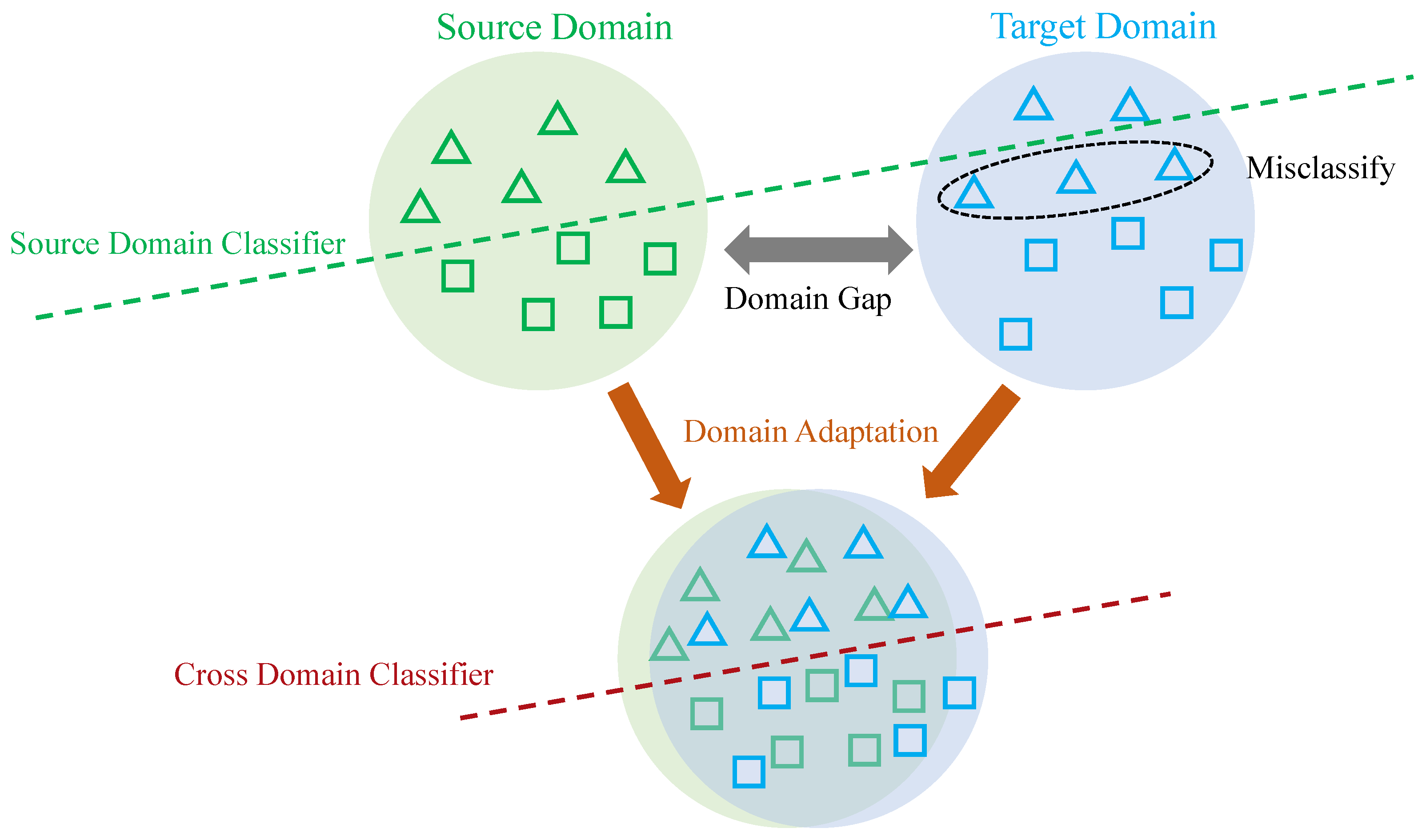
Figure 1. Illustration of source and target data with original feature distributions (top), and new features distributions (bottom) after domain adaptation, where domain adaptation techniques help to alleviate the “domain shift” problem between source and target domains.
2.4. Deep Unsupervised Domain Adaptation
In the concept of domain adaptation, scholars usually refer to the training set as the source domain and the test set as the target domain. Assuming that the model is trained with data collected at the arm (source domain) and later tested with data collected at the leg (target domain), the model does not perform as well. This is because the deep learning model can only recognize test data with the same distribution as the training data. One way to improve the performance of the model in the target domain is to label a large amount of data in the target domain and fine-tune the model trained in the source domain using a supervised approach. However, labeling a large amount of data requires significant human resources.
Domain adaptation (see Figure 1) refers to adapting the model trained in the source domain to the target domain, i.e., reducing the domain gap between the source and target domains and improving the performance of the target domain. Domain adaptation includes semi-supervised domain adaptation and unsupervised domain adaptation. Semi-supervised domain adaptation requires that samples from the target domain are partially labeled. In contrast, unsupervised domain adaptation does not require the target samples to have labels. Deep unsupervised domain adaptation specifically refers to improving the adaptation ability of deep learning models in the target domain. Due to the complexity and nonlinearity of deep learning models, a large number of algorithms for deep unsupervised domain adaptation have emerged in recent years, including mapping-based algorithms, adversarial learning-based algorithms, etc.
This entry is adapted from the peer-reviewed paper 10.3390/s22155507
This entry is offline, you can click here to edit this entry!