In 1986, the heuristic method [31] A* was proposed, which consists of dividing the known area into individual cells and calculating the total cost of reaching the target for each of them. Given the total distance from the starting point to the currently analysed cell and the distance from the analysed cell to the target, the total path cost is calculated with the following formula: where:

F(n) is the total path cost;

G(n) is the cost of reaching from the starting point to the analysed cell; and

H(n) is the cost of reaching from the analysed cell to the target.

The A* algorithm focuses on finding the shortest path to a destination in the presence of static obstacles assuming that both the environment and the location of the obstacles are known. In this method, however, an increased amount of computation is needed for large areas analysis or areas with many obstacles. This significantly increases the path planning time. For the marine vehicles, AUVs and autonomous surface vehicles (ASV), the A* algorithm method is in most cases used in combination with the visibility graph algorithm [32,33,34]. In [35], simulations of two grid-based methods in the 3D environment were compared. Compared to the Dijkstra algorithm, the multi-directional A* proved to be more efficient in terms of the number of nodes and the total length of the path. The practical implementation of this method is associated with the problem of variability of the underwater environment and the lack of precise knowledge about the location of obstacles. Another challenge for practical implementation of this method in AUV may be the unforeseen effect of sea currents.

The artificial potential field (APF) method has its origins in 1986 [36] and assumes the presence of a repulsive field around the obstacle and an attractive area around the target that affect a moving vehicle (e.g., AUV). As a result of the interaction of these virtual fields, the resultant force is determined according to which way the vehicle is moving. In this method, prior knowledge of the environment and the location of obstacles is not needed. It can be used regardless of whether the obstacles in the environment in which the AUV is moving are static or dynamic and whether they have regular or irregular shapes. The crucial condition for this algorithm to be efficient is accurate obstacle detection. The advantage of the APF method is the ease of implementation and low computational requirements, which makes it possible to control AUVs and avoid collisions in close to real time. Despite the many abovementioned advantages, the possibility of local minima or trap situations is considered as a significant disadvantage [37]. Under certain conditions, e.g., a U-shaped obstacle, when the resultant force acting on the AUV is balanced, the algorithm will control the movement of the AUV in a closed infinite loop without reaching the goal. In addition, the passage of the AUV between closely spaced obstacles may not be possible or cause oscillation due to the alternating influence of force fields from opposing obstacles [37,38]. Also, the AUV tends to demonstrate unstable movements when passing around obstacles. In order to solve the local minima problem, APF is combined with other methods, such as [39,40]. In the simulation-based study [41] for AUVs a solution was proposed based on the introduction of a virtual obstacle in the place where the local minimum occurs. Another way to avoid a trap situation can be by using random movements to lead the AUV out of the adverse area (randomised potential field) [42]. Despite the limitations of this method, it is used to control a swarm of robots [43,44,45,46]. Simulation-based studies also prove the possibility of controlling multi-AUV formations [47] and its application in mission planners [48]. In [49], the potential field-based method was used in the practical implementation in NPS ARIES AUV in a real-world environment. To avoid the negative impact of APF method limitations in real implementations, it is necessary to use the global path-planner module based on, e.g., heuristic methods.

Introduced in 1998 [50], the motion-planning algorithm named rapid-exploring random tree (RRT) is a sampling-based method. Any node in the spatial is randomly determined from the initial point (Figure 1). Then, depending on the given direction of movement and the maximum length of the section from the analysed point, the intermediate node is determined. The longer the sections’ connecting nodes, the higher the risk of moving in the wrong direction for a long time and encountering obstacles on the designated path. If any obstacle is detected between waypoints, further route calculation in that direction is ignored. If no obstacles are detected, a random point in the spatial is determined, followed by a new intermediate point.

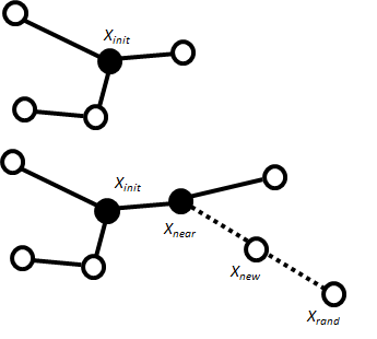
As a result of subsequent iterations (time steps), new edges and path points are determined. The method is easy to process and ensures the finding of a collision-free path (if there is one) in an unknown environment, both 2D and 3D. RRT can be used in both static and dynamic environments [51]. A modification of this method was used in the SPARUS-II AUV and tested in a real-world environment [52]. The study [53] shows the validity of the modified RRT* algorithm for mapping in a 3D environment for multiple AUVs. In [54], an RRT-based approach was used to solve the problem of local minima in the fast warm starting module in the Aqua2 AUV. It was noted that this method is not always efficient in an environment where the path to the target leads through a narrow opening or gap. Another limitation of this method is the need to provide information about large areas of the environment, which is not always possible in practical implementations due to the technical limitations of sensors [55,56,57]. Additionally, the calculated path is suboptimal [58] which requires the use of additional optimisation algorithms.

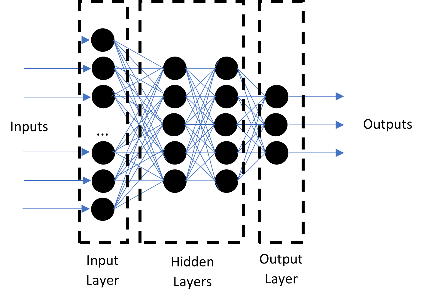
An artificial neural network (ANN) is a machine learning method based on the mathematical mapping of information processing by the human brain. The general structure consists of three layers: input layer, hidden layers, and output layers (Figure 2). The neurons in each layer are connected to all the neurons in the neighboring layer and process the inputs based on the weights in between. The data from each neuron in the input layer multiplied by weights is sent as input to hidden layers where each neuron is assigned a value (bias). Depending on the activation function and bias value, only neurons with a value higher than the threshold value are activated. The output from each layer is also the input for the next layer. The data transfer between the layers is performed only by active neurons. The ANN method requires learning, i.e., indicating the accuracy of the output data. Based on the determination of the expected results, the neural network adjusts the weights between the individual neurons in each iteration in such a way that the output data is as close to the expectations as possible.

The method has learning ability and is applicable in systems that implement complex functions, supporting many outputs based on data from multiple sensors. The algorithm is also efficient for the systems where the input data is incomplete or distorted, or in cases in which there poorly modelled, nonlinear dynamical systems [59,60,61]. The main drawback of this algorithm is the need for long-term training to achieve satisfactory results [62]. In the case of practical implementation for AUV, online learning does not bring satisfactory results due to slow learning speed and long training time [63]. Therefore, offline training for controllers is essential before the AUV can be used in a real-world environment. Reference [64] presents a collision-avoidance controller for static and dynamic obstacles based on neural networks that do not require training. The resulting behaviour of the AUV was defined by neuron weights. It should be noted, however, that this type of controller is suitable for simple AUV operational cases. In [65], the neural network method was used in real implementation in AUV-UPCT. The vehicle required prior learning in ROV mode. In [66], the neural network algorithm was used in a simulation study to control and avoid collisions for multiple AUVs in a 3D environment. In [67], the neural network was used to process real images of the underwater environment (simple, coloured monocular camera) to determine the free space enabling the escape of the AUV from the cluttered environment.

Genetic algorithm (GA) refers to research and optimisation methods inspired by the natural evolution process where only the fittest organisms have a chance for survival. In general, the algorithm starts looking for a solution to a problem by generating a random population of possible solutions. Depending on the applied function, a selection is made during which the least suitable solutions are eliminated [68]. For path planning, the main criterion is the energy cost required to run each path [69]. Then, through an operation called crossover, further potential solutions to the problem (offspring) are created, combining the best solutions from the previous generation (parents). Additionally, in the mutation process, random modifications of the best solutions are created. Then, the GA runs the selection again, adding to the population’s successive possible solutions that are closer and closer to the correct result until a specific final condition is reached, e.g., the number of generations. The main advantage of the GA method is the possibility of fast and global stochastic searching for optimal solutions [70]. In addition, the algorithm is easy to implement and can be used to solve complex problems, such as determining the optimal AUV path in the presence of static and dynamic obstacles in the underwater environment. Due to the random nature of searching for solutions, the algorithm reduces the risk of the local minima problem [71]. In general, the method does not require large numbers of calculations to solve the path-planning problem. However, the route may be suboptimal if too few generations are executed. As the number of generations increases, the route becomes closer and closer to the optimal one due to the constant elimination of the least optimal solutions in the population. It entails an increase in computational costs. Similarly, in a rapidly changing environment or when the environment is very extensive, the amount of computation needed to determine a solution increases significantly. In [69], a modification of the GA was presented in order to determine the energy’s optimal path. The modification involved the introduction of iterations consisting of additional runs of the algorithm with different initial conditions and the operator based on the random immigrants’ mechanism, which sets the level of randomness of the developing population. Reference [72] discussed the framework of the collision-avoidance system based on the GA. The simulation test proved the proper functioning of the method for static and dynamic obstacles. Improved GA was also used in a simulation-based study [73] to optimise energetic routing in a complex 3D environment in the presence of static and dynamic obstacles. The algorithm with improved crossover and mutation probability and the modified fitness function was tested in simulation [70] in comparison with the traditional GA method. The simulation confirmed that the improved GA allows a shorter and smoother path with fewer generations. The method worked very well in the energy optimisation of routing. It should be noted that the efficiency of this method in real testing depends on the correct detection and determination of the obstacle location as well as the target.

The fuzzy logic (FL) method [74,75] is based on the evaluation of the input data depending on the fuzzy rules which can be determined by using the knowledge and experience of experts. In AUV obstacle avoidance systems, the fuzzy controller sensor processes data containing information about the surrounding environment and makes decisions based on it. Then, appropriate signals are transmitted to the actuators. The first stage of the algorithm’s operation is fuzzification, i.e., assigning the input data to the appropriate membership function. Each of the functions is based on a descriptive classification of the input data, e.g., low, medium or high collision risk. Then, in the fuzzy inference process, a data evaluation is performed based on “if prerequisite then result” statements rule. Ultimately, the defuzzification process determines specific system output values (e.g., actuator control signal values). The method can be used for both static and dynamic obstacles. However, when an AUV operates in an unknown environment, the usability of the algorithm directly depends on the implemented rules, and therefore also on the knowledge and experience of experts. The main advantage of the algorithm is its usability in the case of incomplete information about the environment, even containing noises or errors [76]. The method is easy to implement and provides satisfactory results in real-time processing but requires a precise definition of membership functions and fuzzy rules [77]. Additionally, as the number of inputs increases, the amount of input data necessary for the system to process increases. An important issue affecting the effectiveness of the algorithm is also the AUV speed and the complexity of the environment. A fuzzy system usually has at least two inputs. In a very dynamic environment, the use of additional inputs can increase the efficiency of the controller [78]. In some cases, the necessity of performing complex maneuvers to avoid a collision may cause the AUV to be diverted far from the optimal path. For this reason, it is necessary to use additional algorithms that control the path in terms of energy. A simulation study [71] showed that the use of GA to optimise fuzzy logic path planner allows one to achieve greater efficiency and reduce cross-track errors and total traveled path. A modification of this method was also used in a practical implementation in a study [79] where the Bandler and Kohout product of fuzzy relations was used for preplanning in horizontal plane maneuvers. The fuzzy logic method was also used in [80] to control a single unmanned surface vehicle (USV) and in the simulation [81] to control virtual AUVs in the leader–follower formation of AUVs.

The reinforcement learning (RL) method is based on research about the observation of animal behaviour. As a result of strengthening the pattern of behavior by receiving a stimulus by the animal, it increases the tendency to choose actions [82]. Machine learning based on this idea was very intensively developed in the second half of the 19th century. Depending on the requirements of the environment model, the simplicity of data processing, and the iterative nature of calculations, several methods of solving RL problems have been developed, e.g., dynamic programming, Monte Carlo methods, and temporal difference learning. The most crucial method of solving RL problems is the temporal difference method. Depending on the occurrence of the policy function, it is divided into several algorithms, e.g., Actor-Critic, Q-learning or Sarsa method [82]. The actor-critic method consists of autonomous learning of the correct problem solving depending on the received reward or punishment. By performing action, the agent influences the environment by observing the effects of the action. Depending on the implemented reward function, different ways of influencing the environment are assessed. The objective of this method is to learn how to perform such actions in order to get the greatest reward. In the case of path planning, the agent will receive the greatest reward if moving toward the given destination. In general, an agent includes a combination of neural network’s actor and critic. The interaction between them is a closed-loop learning situation [83]. The actor chooses the action for performing to improve the current policy. The critic observes the effects of this action and tries to assess them. The assessment is then compared with the reward function. Based on the error rate, the critic network is updated to predict actor network behaviour in the future better. The abovementioned approach was used in [84] to control four robots. Each of them was able to avoid collisions with other robots and with obstacles. In the study [85], the RL approach was used in a two-dimensional simulation of cooperative pursuit of unauthorized UAV by using a team of UAVs in an urbanized environment. In [86], a simulation of smart ship control algorithm was presented. Moreover, in simulation studies [87,88] the RL approach was used for path planning and motion control of AUVs. The method can be used for both static and dynamic obstacles in an unknown environment. It is characterised by a strong focus on problem solving and shows high environmental adaptability. The RL algorithm can learn to solve very complex problems as long as the correct reward function is used. The inability to manually change the parameters of the learned network is considered as the main drawback of this method. To change the operation of the algorithm, the network must be redesigned, and a long learning process must be performed. Also, checking this method’s operation by simulation does not guarantee its correct operation in a real-world environment.