Recurrent neural networks (RNN) have been shown to outperform other architectures when processing temporally correlated data, such as from wireless communication signals. However, traditional usage assumes a fixed observation interval during both training and testing despite the sample-by-sample processing capabilities of RNNs. Rather than assuming that the testing and observation intervals are equivalent, the observation intervals can be “decoupled" or set independently. This opens the door for processing variable sequence lengths in inference by defining a decision criteria. "Decoupling" can potentially reduce training times and will allow for trained networks to be adapted to different applications without retraining -- including applications in which the sequence length of the signal of interest may be unknown.
1. Decoupling Training and Testing Sequence Lengths
The inherent sample-by-sample nature of recurrent neural networks (RNN) allows training and testing sequence lengths to be set independently. This “decoupling” relaxes the assumption of equivalent input sequence lengths that has previously been used and allows for the potential of greater flexibility between training and inference. Consider a network that is trained on short, fixed observation intervals due to limited time for dataset collection. When the network is deployed, it may need to process signals that are longer than it ever saw in training. Similarly, a network trained for an application with one sequence length should be able to be applied to an equivalent application with a different sequence length—without retraining the network. Ref.
[1] addressed this problem for convolutional neural networks (CNN) by processing multiple, fixed observation intervals and fusing the results. However, with RNNs, a variable sequence length can be easily processed with no changes necessary to the architecture. The flexibility of RNNs make them preferable for some applications.
In general, longer sequence lengths—in either training or testing—will result in improved performance
[2][3]. However, a thorough analysis of the impact of training and testing sequences—individually and combined— is still necessary. In particular, the impact of sequence length on network bias and generalization to data outside the original training range needs to be considered. By examining the trends of training and testing sequence lengths, the most advantageous sequence length for a problem set can be selected—potentially reducing training time and network complexity and allowing for increased flexibility in deployment.
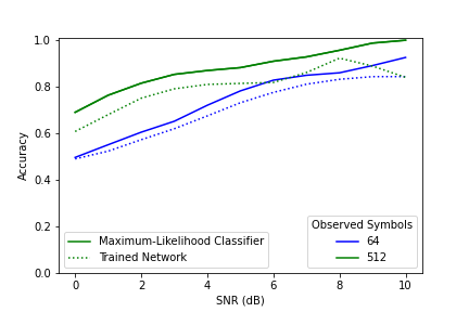
Figure 1: A comparison between the maximum-likelihood classifier and an RNN based AMC trained on 64 symbols.
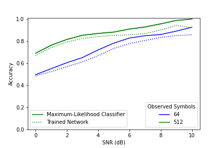
Figure 2: A comparison between the maximum-likelihood classifier and an RNN based AMC trained on 512 symbols.
Figures 1 and 2 show a comparison between the maximum-likelihood classifier (ML) and two RNN based automatic modulation classifier (AMC) -- one trained on 54 symbols and the other trained on 512 symbols. The ML classifier -- under ideal conditions -- forms the upper bound on classification accuracy for a particular number of observed symbols. The network trained on 64 symbols and tested on 512 symbols was able to achieve accuracy higher than the performance bound for 64 symbols. This shows that a trained AMC's accuracy is bounded by the number of symbols observed in testing rather than the number seen in training. While the number of observed symbols is what ultimately bounds the network performance, the number of symbols used in training is still relevant. Notably, the network trained on 512 symbols achieved performance closer to the ML classifier than the network trained on 64 symbols– even though both observed 512 symbols in training. A training sequence length much shorter than the one used in testing may result in decreased performance.
Examining a more complex case with frequency offset and varied oversampling rates showed that some networks had diminishing returns when testing on sequence lengths much longer than they were trained on. To gain a better understanding of this behaviour the impact of several different parameters was examined. Of particular interest was an examination of how training sequence length impacted network bias and generalization to data outside the training range. As networks trained on shorter sequence lengths observe fewer symbols in training, there were concerns that they would be more likely to develop a bias. However, there was no clear trend found between training on a shorter sequence length and a higher likelihood of network bias. Despite this, bias is still impacted by sequence length. When testing a biased network on a longer sequence length – regardless of the sequence length used in training – the bias actually becomes more apparent.
Examining network performance across each modulation scheme also provided some insight into the saturation observed. For the networks trained on a short sequence length, performance did not increase evenly across all signal types. Instead as the testing sequence length increased, the network began to prefer certain classes over others. In contrast, the network trained on a long sequence length saw performance improvement for all classes. While this may seem to be simply the result of a biased network, the network was not biased as it was not choosing one class to the detriment of another. In the biased networks that were examined, performance for some classes actually saw a significant decrease – in this case it simply stays the same. Ultimately, this suggests that the networks trained on a smaller sequence length did not adequately learn to identify each modulation. As a result, they were unable to generalize to longer sequence lengths.
Testing the networks on data outside the training range showed similar results. Networks trained on shorter sequence lengths were unable to generalize to unseen data. In contrast, networks trained on longer sequence lengths saw significant improvement in performance when sequence length increased – even for data outside the training range. The goal of “decoupling" was to allow the testing and training sequence length to be set independently rather than assuming them to be equivalent. However, they are not truly independent. To achieve the best performance the training sequence length should be chosen so that it is as close as possible to the sequence lengths that will be seen in testing. In cases where the testing sequence length is unknown or variable, the best choice of training sequence length will depend on the complexity of the problem. A smaller training sequence length will save time in both data collection and network training. However, it comes with an increased risk of capping network performance due to insufficiently training the model to generalize to longer sequence lengths. The advantage of training on a longer sequence length increases with the complexity of the problem.
2. Managing Variable and Unknown Sequence Lengths in Inference
In many cases, the sequence length in inference may be variable or completely unknown. Rather than setting a fixed testing sequence length it would be preferable to allow for variable sequence lengths to be processed. Such an approach is commonly used in machine text translation where the network will process inputs until it displays an <EOS> (end of sentence) key [4] . However, in spectrum sensing applications the choice of appropriate evaluation lengths is not nearly as obvious—especially with limited or no prior knowledge of the signals of interest. While pre-processing steps could be added to identify and separate the signal prior to feeding it into the network, this would not be ideal for applications that are time sensitive.
The true utility of RNNs is the ability to easily process a variable number of samples. As a result they can be trained on varying sequence lengths and evaluated for any arbitrary number of input samples.
Since simpler input formats with good channel propagation conditions (higher signal-to-noise ratios, lower frequency offsets, simpler modulation schemes, etc.) may require lower sequential data needs to make a reliable decision, a flexible stopping condition would be preferable. Consider that in Ref.
[5], an RNN based AMC network was trained on three separate sequence lengths determined by the oversampling rate. Signals that had a higher oversampling rate needed to be processed for additional samples in order to see the same number of symbols. However, it was unclear how this would be approached when the oversampling rate of an input signal is unknown. Ref.
[6] recognized the potential for real-time classification with LSTMs by training the classifier only on the final hidden state of an LSTM autoencoder. The new training process significantly reduced training time. It also allowed for faster real-time classification as only the LSTM operations were repeated at each time step. However, the authors did not address how to determine a when an accurate decision has been reached.
Ref. [7] introduces a potential approach called “just enough" decision making (JED). The idea is that an RNN can be made more efficient by stopping its processing of new inputs once it is sufficiently confident in its decision. This is a separate concept from “early-stopping" which aims to prevent overfitting by stopping network training when certain criteria are met. In JED, no changes are currently made in the training stage – instead all analysis is carried out during inference with the decision criteria being examined at each time step. If the decision criteria is met, then the final output is returned and no further inputs are processed. The delta-threshold (DEL) technique is a decision criteria designed to look for stability in the neural network’s output softmax value by examining its change over each input.
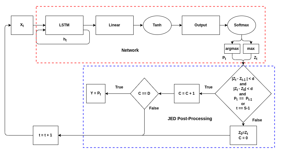
Figure 3: A diagram of the JED process for a single time-step. Note that d is the delta-threshold, D is the duration, and S is the maximum number of samples that can be processed.
Figure 3 shows an overview of the DEL technique for a single time-step. The technique depends on two user-defined variables: delta-threshold which determines the amount of change between outputs that is tolerated and duration, the number of consecutive inputs for which the change must be below the delta-threshold. Two change values are used. The first is the change between the current input and the first input in the series. The second is the change between consecutive inputs. For example, if duration is 100, the delta-threshold is 0.1, and the first sample in the series has a softmax output of 0.9 for a given class, then the output of the network must stay between 0.8 and 1 for that class for 100 samples. Additionally, the change between consecutive samples must not exceed 0.1; if the output drops from 0.97 to 0.8, the counter will reset. The network will only make its decision if both these conditions are true for the highest class for 100 consecutive samples. However, to prevent the network from processing samples for an infinitely long time, a maximum number of samples to process was added. If the network has not made a decision by the time 2048 samples have been processed, it will output the current decision.
In general, the JED method processes simpler signals for shorter sequence lengths. However, when the method saw data that had a lower SNR than seen in training, different networks gave different responses. Networks trained on shorted sequence lengths had poor generalization and were confidently incorrect. As a result, the average number of samples processed decreased even though the problem was more difficult. Networks trained on longer sequence lengths had better generalization, so the average number of samples processed continued to increase as SNR decreased. However, despite this, accuracy for the latter networks did not really improve. Twice as many samples were processed on average, but performance was still barely above random guessing. Relinquishing direct control of the sequence length can result in processing many more samples with no real benefit. This problem can be minimized by choosing an appropriate value for the user-defined parameters – particularly the maximum sequence length.
The user-defined parameters can also be “tuned" based on the application. The two combinations used in testing were chosen to get maximum accuracy, however, in other applications it may be preferable to instead further reduce the number of samples processed. The first combination tested improved accuracy by almost 7% over a fixed sequence length of 1024 samples while processing a similar number of samples on average. The second combination tested improved accuracy by 4% over a fixed sequence length of 2048 while processing around 500 fewer samples on average.
The JED method provides a useful decision criteria for applications where the signal length in inference is unknown or variable. It can also be beneficial for time-sensitive applications like electronic warfare and dynamic spectrum access. However, it is most useful when there is significant variation in the input data. If some signals are significantly easier to identify than others, using JED post-processing can result in both higher accuracy and fewer samples processed on average. However, using JED relinquishes direct control of the number of samples processed which may not be desirable in some applications.
This entry is adapted from the peer-reviewed paper 10.3390/s22134706