Your browser does not fully support modern features. Please upgrade for a smoother experience.
Please note this is an old version of this entry, which may differ significantly from the current revision.
Passive infrared optical gas imaging (IOGI) is sensitive to toxic or greenhouse gases of interest, offers non-invasive remote sensing, and provides the capability for spatially resolved measurements. It has been broadly applied to emission detection, localization, and visualization.
- infrared optical gas imaging (IOGI)
- emission quantification
- artificial intelligence (AI)
1. Introduction
Toxic emissions from thermal engines in the power generation sector have been the cause of serious societal concern [1], especially as they relate to greenhouse gases contributing significantly to global warming [2], which is currently the main focus of international environmental protection policies. Accurate measurement is the foundation of effective emission control and, consequently, the development of advanced, smart, and convenient emission quantification tools emerges as a pressing technical necessity [3].
Pursuing such measurements in the infrared (IR) band offers the advantage that they can directly quantify the global warming potential of gaseous emissions. Most interesting combustion species, such as hydrocarbons and species containing the C-H bond in general, including carbon oxides and nitric oxides, all have strong signals in the infrared range [4], as shown in Table 1. It is also noted that nitrogen and oxygen, which make up the majority of air, do not have IR activity because they are homonuclear diatomics, meaning there is no such interference. On the other hand, it is true that, especially in a combustion environment, IR signals are vulnerable to broad-band black body emission from high-temperature particles [5,6], whereas the puzzling emission spectrum of water vapor constitutes another source of interference [4,7].
Table 1. Absorption bands of several pollutants at the International Standard Atmosphere (ISA).
|
Molecule |
Absorption Wavebands (µm) |
Molecule |
Absorption Wavebands (µm) |
||
|---|---|---|---|---|---|
|
CO |
2.29–2.48 |
4.36–5.05 |
NO |
2.63–2.78 |
5.03–5.78 |
|
CO2 |
2.66–2.81 |
4.07–4.43 |
NO2 |
3.38–3.53 |
5.92–6.57 |
|
CH4 |
3.07–3.71 |
6.67–9.09 |
SO2 |
3.94–4.07 |
6.94–9.44 |
Infrared optical gas imaging (IOGI), which involves the use of infrared imagers or infrared spectral cameras in order to generate images [4,8,9,10], has attracted considerable attention since the recent advances in the development of cost-effective, IR-sensitive chips [11,12,13,14]. Contrary to the well-developed field of infrared spectroscopy [15], IOGI is a multidimensional, spatially resolved measurement. This kind of optical-field measurement provides the possibility for the determination of the geometrical characteristics of pollutant dispersion. From an engineering application perspective, laser-based spectroscopy measurement has a higher cost and requires complex data interpretation by highly skilled users [16], which makes its application to industrial practice challenging. As a result, a recent comparative assessment of various optical measurements by the U.S. Environmental Protection Agency (EPA) [17] recognizes only OGI as a work practice that can be a potential alternative for the Leakage Detection and Repair (LDAR) techniques, which are currently dominant in industrial practice and are based on sampling (through “sniffers”) and ex-situ gas analysis with ionization detectors.
IOGI has now been applied in emission detection, location, and visualization. De Almeida et al. [18] reported using portable infrared cameras to detect and visualize the volatile organic compounds (VOC) leakage of four floating production, storage, and offloading facilities of a deep-offshore field in Angola. Moreover, Lyman et al. [19] used both aerial and ground-based IOGI to detect hydrocarbon emissions of more than three thousand oil and gas facilities in the Uinta Basin and reported that aerial scanning could observe the emission of 81% of gas wells, while the ground-based method could reach up to 90%. In addition, Furry et al. [20] assessed the performance of IOGI by detecting the fugitive gas leakage of six refineries which had a total of 110,000 components. In their test, they were able to scan 4500 components per hour on average and detect leakages with a minimum detection limit of 11 g per hour. They concluded that IOGI had comparable accuracy to conventional LDAR but was more efficient [21]. Because of its potential advantages in terms of high efficiency and remote sensing, IOGI has been termed a “smart” LDAR [22].
Despite these successful detection applications, the potential of utilizing IOGI for emission quantification is only starting to be explored. Some initial registries of related work have already appeared. For example, the EPA has collected information from various types of spectral cameras and recorded applications of spectral imagers for measurements of emission concentrations [23]. Additionally, Fox et al. [24] suggested the utilization of dispersion models to measure emission rates. More recently, Hagen [25] has summarized various technologies based on spectral imagers to measure column density, concentration, and emission rates.
2. Challenges in IOGI Emission Quantification
Using IR cameras to quantify emissions is recognized as a tough task. In [23], EPA claimed that the “thermal IR camera’s major drawback is its inability to measure the quantity or concentration of gas present in a gas plume”. Fox et al. [24] stated that “most current OGIs only present a qualitative (visual) flux estimate”. Hagen [25] also mentioned that “while infrared cameras have proven useful in detecting leaks, their use in quantifying leaks has only recently been analyzed, and is the subject of ongoing research”. Even the newest AI-assisted OGI system developed by FLIR, one of the top infrared camera manufacturers, can only be used for intelligent gas detection and segmentation [26].
On this condition, EPA recommends using ancillary devices for emission quantification after OGI detects and locates the emission [27]. Following this idea, Ravikumar et al. [28] used the emission factor method [29] and the Hi-Flow sampler [30] to calculate the emission rate. Almeida et al. [18] adopted an infrared gas analyzer to analyze the gas composition and concentration, Al-hilal et al. [31] utilized flame ionization detectors (FID) or photoionization detectors (PID) for gas concentration measurement, while Gal et al. [32] utilized multiple devices, i.e., infrared gas analyzer, micro-chromatography, and the accumulation chamber technique, to quantify gas concentrations and flux. In addition to utilizing sniffer and ex situ gas analyzers, Englander et al. [33,34] applied laser absorption spectroscopy (LAS) [15] to quantify column concentration. Furthermore, Lev-On et al. [22] summarized all these OGI-assisted quantification methods into five categories, i.e., the average expected, leak/no leak, random sample screening, periodic screening, and high leaker sniffing.
Figure 1 shows the simple three-layer radiative transfer modeling for IR imaging [35]. The radiation sensed by the camera is the integrated emission from three layers: background, gas cloud, and foreground. Part of the radiation is also absorbed when crossing these three layers. To simplify the analysis, scattering and reflection are ignored.
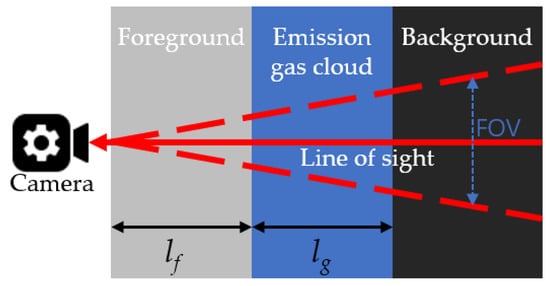
Figure 1. Three-layer radiative transfer modeling for passive OGI.
Suppose each layer is homogenous, absorbs some radiation from the prior layer, and emits radiation as well. The radiation intensity at the exit of each layer can be expressed as follows:

where I is the radiative intensity (W/(m2⋅sr)), the subscripts v,o,e and t represent the frequency of the light wave, the output of the layer, emission of the layer, and transmission of the layer, respectively.


According to the Beer–Lambert law, transmissivity can be expressed as:
where t is the transmissivity, kv is the absorption coefficient (cm−1), and l is the light path length of the layer (cm). Meanwhile, the sum of transmissivity and absorptivity is 1 when scattering and reflection are neglectable, that is:
where αv is the absorptivity. Supposing all three layers are in thermal equilibrium, and following Kirchhoff’s law of thermal radiation that emissivity equals absorptivity, the researchers substitute Equations (2) and (3) into Equation (1):
where Iv,B is the black body radiation, Iv,i is the radiation intensity at the incident surface of the layer. Blackbody radiation can be modeled by Plank’s law as:
where h is the Plank constant, kB is the Boltzmann constant, c is the light speed, and T is the temperature. Then, the absorption coefficient, kv, of gas species j could be calculated from:
where s is the line intensity per molecule (cm−1/(molecule⋅cm−2)), which is a function of temperature, ϕv is the line shape function [36] (cm−1), which is a function of both pressure and temperature, P is the local pressure (Pa), and X is a mole fraction. The total absorption coefficient can be simplified as the sum of the absorption coefficients of each species:
In practice, a bandpass filter is used to select the target gas species, so Equation (7) can be simplified as follows:
where subscript t represents the target gas, therefore, combining Equations (4)–(8), Equation (4) can be rewritten as:
The mole fraction Xt is coupled with the light path length l. Using the ideal gas equation of the state, Xtl, can be transformed as the product of concentration Ct and light path length l, which is called column density [25,37] and can be expressed as follows:
where CLt, Mt and Ct are the column density, molecular mass, and concentration of target gas, respectively. The final intensity at each pixel is a function of the camera characteristics and double integration of the camera incident intensity at all wavelengths of the band and the covered surface of the pixel, i.e.,
where Ip is the pixel value, f symbolizes a functional relationship, Iv,c is the camera incident light strength at the wavelength inside the filtered waveband, dA is a finite element of the surface that a pixel covers, and D


represents the camera characteristics of transforming radiation into pixel charge and includes chip-sensing efficiency, transforming efficiency, and noise characteristics.
In most cases, pressure can be supposed to be constant along the optical path. After accumulating the transmission and absorption of three layers, the pixel value can be represented as follows:
where Rb is the background radiation, CLg and CLf are the column densities of the target gas substance in gas cloud and foreground, respectively, Tf and Tg are the temperatures of the gas cloud and foreground, respectively, D is the device characteristics, and ε is the noise that comes from the environment and devices, such as wind effect, scattering, etc., which can be neglected and regarded as measurement uncertainty. Parameters Rb, CLf, Tf, D and ε can be summarized as environmental factor εe as they are controlled by the environment and measurement devices and are in general considered constant for the experimental condition. Thus, for a given imager, Equation (12) can be simplified and rewritten as:
Consequently, column density is the function of Ip,Tg, εe, that is:
Equations (13) and (14) reveal two important insights. First, from the pixel value of an IR image, we cannot decouple the concentration and light path length—they are represented by column density. Second, the fundamental quantitative parameter, column density, is a function of three parameters, i.e., pixel value, gas temperature, and environmental factors (Rb, CLf, Tf, D and ε ). Therefore, a single pixel value is not sufficient to retrieve column density.


3. Column Density Quantification
Since extracting column density from a single pixel is impossible because the pixel value is also affected by the temperature of the gas cloud and the environmental factor εe, as shown, additional information is needed in order to extract quantitative information. Depending on what kind of information is added, existing column density quantification methods can be divided into two classes, i.e., elimination and augmentation.
In the elimination method, the idea is to eliminate the influence of temperature and environmental factors so that the relationship between column density and pixel value can be fixed, that is,
The concept of the augmentation method is to add spectral information to each pixel, that is, spectral imaging, a combination of spectroscopy and imaging, so that the image conveys temperature information as well, in a latent way. The problem then transforms to column density quantification from the spectral information at each pixel, i.e.,
where v is the frequency, Bg is the characteristic band for the target gas, and SP is the spectrum obtained at a given pixel, which is a wavenumber function.
4. Concentration Quantification
According to the definition of column density, concentration can be decoupled from the column density estimated with the methods discussed above once the light path length is known. In other words, coupling gas cloud geometry information with column density can provide a pixel-level concentration measurement. Those techniques where the emphasis is to acquire light-path length are categorized as geometry acquisition-based methods. On the other hand, machine learning algorithms can be used in order to estimate concentration from images captured from a designated object, such as a burner or a flare. Using machine learning, light path information can be acquired implicitly rather than explicitly as in geometry-acquisition-based methods, since the 2D information (images) of the gas cloud also conveys the 3D geometry of the gas cloud for a given object. Indeed, machine learning methods can learn inverse projection mapping, thus granting access to 3D information. Methods using machine learning algorithms to estimate the emission concentration of a given object directly from 2D images are categorized as machine-learning-based methods.
5. Emission Rate Quantification
In addition to concentration, the actual mass flow rate of emissions is also a technically very relevant quantity. The methods to estimate emission rate can be roughly divided into two categories: (i) propagation-speed-based method and (ii) minimum-detectable-concentration-based method. If the concentration is known via the methods that have been described in previous sections, the missing information in order to determine mass flow rate is propagation speed, which is the focus of propagation-speed-based methods. However, there are also technologies, the emphasis of which is on the use of the minimum detectable concentration in order to replace the active measurement of column density/concentration, and this parameter is further used to estimate the emission rate. These technologies are categorized as minimum-detectable-concentration-based methods here.
This entry is adapted from the peer-reviewed paper 10.3390/en15093304
This entry is offline, you can click here to edit this entry!