Your browser does not fully support modern features. Please upgrade for a smoother experience.
Please note this is an old version of this entry, which may differ significantly from the current revision.
Radar can measure range and Doppler velocity, but both of them cannot be directly used for downstream tasks. The range measurements are sparse and therefore difficult to associate with their visual correspondences. The Doppler velocity is measured in the radial axis and, therefore, cannot be directly used for tracking.
- automotive radars
- radar signal processing
- autonomous driving
1. Depth Estimation
Pseudo-LiDAR-based visual object detection [1][2][3] has become a popular research topic. The core idea is to project pixels into a pseudo point cloud to avoid distortions induced by inverse projective mapping (IPM). The pseudo LiDAR detection is built on depth estimation. Visual depth estimation is an ill-posed problem because of the scale ambiguity. However, learning-based methods, either supervised [4] or self-supervised [5], can successfully predict dense depth maps with cameras only. Roughly speaking, these methods learn a priori knowledge of the object size from the data and are therefore vulnerable to some data-related problems, such as sensitivity to input image quality [5] and learning non-causal correlations, such as object and shadow correlations [6]. These limitations can be mitigated with the help of range sensors, such as LiDAR and radar. Depth completion is a sub-problem of depth estimation. It aims to recover a dense depth map for the image using the sparse depth measured by range sensors. Compared to LiDAR, radar has the advantages of a low price, long range, and robustness to adverse weather. Meanwhile, it faces the problems of noisy detections, no height measurements, and sparsity. As shown in Figure 1, due to multi-path propagation, radar can see the non-line-of-sight highly reflective objects, such as wheel rims and occluded vehicles. In [7], the authors refer to this phenomenon as the see0through effect. It is beneficial in 3D coordinates, but brings difficulty in associating radar detections with visual objects in image view.
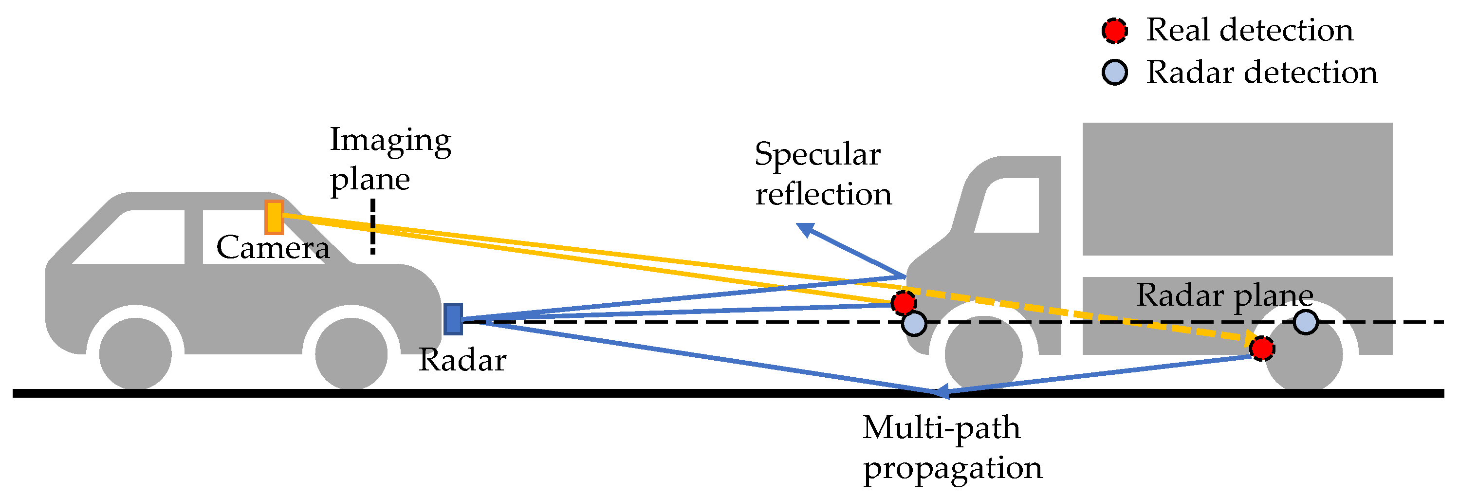
Figure 1. Radar range measurements. Off-the-shelf radars return detections on a 2D radar plane. The detections are sparsely spread on objects due to specular reflection. Due to multi-path propagation, radar can see through occlusions, and meanwhile, this can cause some noisy detections.
The two-stage architecture is widely applied for image-guided radar depth completion tasks. Lin et al. [8] adopted a two-stage coarse-to-fine architecture with LiDAR supervision. In the first stage, a coarse radar depth is estimated by an encoder–decoder network. Radar and images are processed independently by two encoders and fused together at the feature level. Then, the decoder outputs a coarse dense depth map in image view. The predicted depth with large errors is filtered out according to a range-dependent threshold. Next, the original sensor inputs and the filtered depth map are sent to a second encoder–decoder to output a fine-grained dense map. In the first stage, the quality of association can be improved by expanding radar detections to better match visual objects. As shown in Figure 2b, Lo et al. [9] applied height extension to radar detections to compensate for the missed height information. A fixed height is assumed for each detection and is projected onto the image view according to the range. Then, the extended detections are sent to a two-stage architecture to output a denoised radar depth map. Long et al. [10] proposed a probabilistic association method to model the uncertainties of radar detections. As shown in Figure 2c, radar points are transformed into a multi-channel enhanced radar (MER) image, with each channel representing the expanded radar depth at a specific confidence level of association. In this way, the occluded detections and imprecise detections at the boundary are preserved, but with a low confidence. Gasperini et al. [7] used radar as supervision to train a monocular depth estimation model. Therefore, they applied a strict filtering to only retain detections with high confidence. In the preprocessing, they removed clutters inside the bounding box that exceeded the range threshold and discarded points in the upper 50% and outer 20% of the box, as well as the overlapping regions to avoid the see-through effect. All the background detections were also discarded. For association, they first applied a bilateral filtering, i.e., an edge-preserving filtering, to constrain the expansion to be within the object boundary. They further clipped the association map close to the edge to get rid of imprecise boundary estimations. To compensate for height information, they directly used the height of the bounding box as a reference. Considering the complexity of the vehicle shape, they extended the detections to the lower third of its bounding box to capture the flat front surface of the vehicle.

Figure 2. (a) Radar detection expansion techniques. (b) Extend radar detections in height. (c) Build a probabilistic map, where the dark/light blue indicates channel with high/low confidence threshold. (d) Apply a strict filtering according to the bounding box, where only detections corresponding to the frontal surface are retained.
As the ground truth, LiDAR has some inherent defects, such as sparsity, limited range, and holes with no reflections. Long et al. [10] suggest to preprocess LiDAR points for better supervision. They accumulated multiple frames of LiDAR point clouds to improve density. Pixels with no LiDAR reaches are assigned zero values. Since LiDAR and the camera do not share the same FoV, the LiDAR points projected to the image view also have the occlusion problem. Therefore, the occluded points are filtered out by two criteria: one is the difference between visual optical flow and LiDAR scene flow, and the other is the difference between the segmentation mask and bounding boxes. Lee et al. [11] suggest to use both the visual semantic mask and LiDAR as supervision signals. Visual semantic segmentation can detect smaller objects at a distance, thus compensating for the limited range of LiDAR. To extract better representations, they leveraged a shared decoder to learn depth estimation and semantic segmentation concurrently. Both the LiDAR measurement and the visual semantic mask annotations are used as supervision. Accordingly, the loss function consists of three parts: a depth loss with LiDAR points as the ground truth, a visual semantic segmentation loss, and a semantic guided regularisation term for smoothness.
Projecting radar to the image view will lose the advantages of the see-through effect. Alternatively, Niesen et al. [12] leveraged radar RA maps for depth prediction. They used a short-range radar with a maximum range of 40 m. Because of the low angular resolution, the azimuth smearing effect is obvious, i.e., the detections are smeared as a blurry horizontal line in RA maps. It is expected that fusion of the image and RA map can mitigate this effect. Therefore, they used a two-branch encoder–decoder network with the radar RA map and image as inputs. A dense LiDAR depth map was used as the ground truth. Different from the above methods that align LiDAR to the image, they cropped, downsampled, and quantised LiDAR detections to match the radar’s FoV and resolution. The proposed method was tested with their self-collected data. Although the effectiveness of the RA map and point cloud was not compared, it provides a new direction to explore radar in the depth estimation task.
2. Velocity Estimation
For autonomous driving, velocity estimation is helpful for trajectory prediction and path planning. Radar can accurately measure the Doppler velocity, i.e., radial velocity in polar coordinates. If a vehicle moves parallel to the ego-vehicle at a distance, its actual velocity can be approximated by the measured Doppler velocity. However, this only applies in highway scenarios. On urban roads, it is possible for an object to move tangentially while crossing the road, then its Doppler velocity will be close to zero. Therefore, Doppler velocity cannot replace full velocity. Recovering full velocity from the Doppler velocity needs two steps: first, compensate the ego-motion, then estimate the tangential velocity. In the first step, the ego-motion can be estimated by visual-inertial odometry (VIO) and GPS. Radar-inertial odometry [13][14] can also be used in visually degraded or GPS-denied environments. Then, the Doppler velocity is compensated by subtracting the ego-velocity. In the second step, the full velocity is estimated according to the geometric constraints. Suppose that the radar observes several detections of an object and that the object is in linear motion. As shown in Figure 3a, the relationship between the predicted linear velocity and the measured Doppler velocity is given by
where the subscript i denotes the i-th detection and θi is the measured azimuth angle. By observing N detections per object, we can solve the linear velocity using the least-squares method. However, the L2 loss is not robust to outliers, such as clutter and the mirco-Doppler motion of wheels. Kellner et al. [15] applied RANSAC to remove outliers, then used orthogonal distance regression (ODR) to find the optimal velocity.
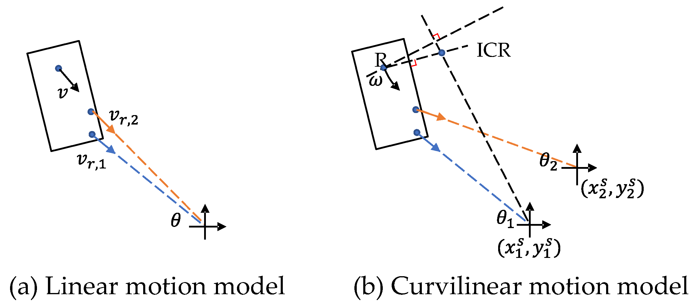
Figure 3. Radar motion model. (a) Linear motion model needs multiple detections for the object. (b) Curvilinear motion model requires either two radars to observe the same objects or the determination of the vehicle boundary and rear axle.
Although the linear motion model is widely used for its simplicity, it will generate large position errors for motion with high curvature [16]. Alternatively, as shown in Figure 3b, the curvilinear motion model is given by
where ω is the angular velocity, θ is the angle of the detected point, (xc,yc) represents the position of the instantaneous centre of rotation (ICR), and (xS,yS) represents the known radar position. In order to decouple angular velocity and the position of the ICR, we need at least two radar sensors that observe the same object. Then, we can transform (2) into a linear form as
where the subscript j denotes the j-th radar. Similarly, RANSAC and ODR can be used to find the unbiased solution of both the angular velocity and position of the ICR [17]. For the single radar setting, it is also possible to derive a unique solution of (2) if we can correctly estimate the vehicle shape. According to the Ackermann steering geometry, the position of the ICR should be located on a line extending from the rear axle. By adding this constraint to (2), the full velocity can be determined in closed form [18].
The above methods predict velocity at the object level under the assumption of rigid motion. However, the micro-motion of object parts, such as the swinging arms of pedestrians, are also useful for classification. Capturing these non-rigid motions requires velocity estimation at the point level. This can be achieved by fusing with other modalities or by using temporal consistency between adjacent radar frames. Long et al. [19] estimated pointwise velocity by the fusion of radar and cameras. They first estimated the dense global optical flow and the association between radar points and image pixels through neural network models. Next, they derived the closed-form full velocity based on the geometric relationship between optical flow and Doppler velocity. Ding et al. [20] estimated the scene flow for the 4D radar point cloud in a self-supervised learning framework. Scene flow is a 3D motion field and can be roughly considered as the linear velocity field. Their model consists of two steps: flow estimation and static flow refinement. In the flow estimation step, they adopted a similar structure with PointPWCNet [21]. To compensate for the positional randomness of detections between frames, a cost–volume layer is utilised for patch-to-patch correlation. The features and correlation maps are then sent to a decoder network for flow regression. In the static flow refinement step, they assumed that most radar detections are static and, therefore, used the Kabsch algorithm [22] to robustly estimate the ego-motion. They then filtered out moving objects based on the coarse ego-motion and applied the Kabsch algorithm again to all static points for fine-grained ego-motion estimation. The self-supervised loss consists of three parts: a radial displacement loss, which penalises errors between the estimated velocity projected along the radial axis and the measured Doppler velocity, a soft Chamfer distance loss, which encourages temporal consistency between two consecutive point clouds, and a soft spatial smoothness loss, which encourages the spatial consistency for the estimated velocities with their neighbours. The soft version of loss is used to model spatial sparsity and the temporal randomness of the radar point cloud.
This entry is adapted from the peer-reviewed paper 10.3390/s22114208
References
- Wang, Y.; Chao, W.L.; Garg, D.; Hariharan, B.; Campbell, M.; Weinberger, K.Q. Pseudo-lidar from visual depth estimation: Bridging the gap in 3d object detection for autonomous driving. In Proceedings of the IEEE/CVF Conference on Computer Vision and Pattern Recognition (CVPR), Long Beach, CA, USA, 15–20 June 2019; pp. 8445–8453.
- Weng, X.; Kitani, K. Monocular 3d object detection with pseudo-lidar point cloud. In Proceedings of the IEEE/CVF International Conference on Computer Vision Workshops (ICCV Workshop), Seoul, Korea, 27 October–2 November 2019.
- Qian, R.; Garg, D.; Wang, Y.; You, Y.; Belongie, S.; Hariharan, B.; Campbell, M.; Weinberger, K.Q.; Chao, W.L. End-to-end pseudo-lidar for image-based 3d object detection. In Proceedings of the IEEE/CVF Conference on Computer Vision and Pattern Recognition (CVPR), Virtual, 14–19 June 2020; pp. 5881–5890.
- Fu, H.; Gong, M.; Wang, C.; Batmanghelich, K.; Tao, D. Deep ordinal regression network for monocular depth estimation. In Proceedings of the IEEE Conference on Computer Vision and Pattern Recognition (CVPR), Salt Lake City, UT, USA, 18–22 June 2018; pp. 2002–2011.
- Godard, C.; Mac Aodha, O.; Firman, M.; Brostow, G.J. Digging into self-supervised monocular depth estimation. In Proceedings of the IEEE/CVF International Conference on Computer Vision (ICCV), Seoul, Korea, 27 October–2 November 2019; pp. 3828–3838.
- van Dijk, T.; de Croon, G. How do neural networks see depth in single images? In Proceedings of the IEEE/CVF International Conference on Computer Vision (ICCV), Seoul, Korea, 27 October–2 November 2019; pp. 2183–2191.
- Gasperini, S.; Koch, P.; Dallabetta, V.; Navab, N.; Busam, B.; Tombari, F. R4Dyn: Exploring radar for self-supervised monocular depth estimation of dynamic scenes. In Proceedings of the 2021 International Conference on 3D Vision (3DV), Prague, Czech Republic, 12–16 September 2021; pp. 751–760.
- Lin, J.T.; Dai, D.; Van Gool, L. Depth estimation from monocular images and sparse radar data. In Proceedings of the 2020 IEEE/RSJ International Conference on Intelligent Robots and Systems (IROS), Las Vegas, NV, USA, 25–29 October 2020; pp. 10233–10240.
- Lo, C.C.; Vandewalle, P. Depth Estimation From Monocular Images And Sparse Radar Using Deep Ordinal Regression Network. In Proceedings of the 2021 IEEE International Conference on Image Processing (ICIP), Anchorage, AK, USA, 19–22 September 2021; pp. 3343–3347.
- Long, Y.; Morris, D.; Liu, X.; Castro, M.; Chakravarty, P.; Narayanan, P. Radar-camera pixel depth association for depth completion. In Proceedings of the IEEE/CVF Conference on Computer Vision and Pattern Recognition (CVPR), Virtual, 19–25 June 2021; pp. 12507–12516.
- Lee, W.Y.; Jovanov, L.; Philips, W. Semantic-guided radar-vision fusion for depth estimation and object detection. In Proceedings of the 32nd British Machine Vision Conference (BMVA), Virtual, 22–25 November 2021; p. 13.
- Niesen, U.; Unnikrishnan, J. Camera-Radar Fusion for 3-D Depth Reconstruction. In Proceedings of the 2020 IEEE Intelligent Vehicles Symposium (IV), Melbourne, VIC, Australia, 7–11 September 2020; pp. 265–271.
- Kramer, A.; Stahoviak, C.; Santamaria-Navarro, A.; Agha-Mohammadi, A.A.; Heckman, C. Radar-inertial ego-velocity estimation for visually degraded environments. In Proceedings of the 2020 IEEE International Conference on Robotics and Automation (ICRA), Virtual, 31 May–31 August 2020; pp. 5739–5746.
- Cen, S.H.; Newman, P. Precise ego-motion estimation with millimetre-wave radar under diverse and challenging conditions. In Proceedings of the 2018 IEEE International Conference on Robotics and Automation (ICRA), Brisbane, Australia, 21–25 May 2018; pp. 6045–6052.
- Kellner, D.; Barjenbruch, M.; Dietmayer, K.; Klappstein, J.; Dickmann, J. Instantaneous lateral velocity estimation of a vehicle using Doppler radar. In Proceedings of the 16th International Conference on Information Fusion (FUSION), Istanbul, Turkey, 9–12 July 2013; pp. 877–884.
- Schubert, R.; Richter, E.; Wanielik, G. Comparison and evaluation of advanced motion models for vehicle tracking. In Proceedings of the 2008 11th International Conference on Information Fusion (FUSION), Cologne, Germany, 30 June–3 July 2008; pp. 1–6.
- Kellner, D.; Barjenbruch, M.; Klappstein, J.; Dickmann, J.; Dietmayer, K. Instantaneous full-motion estimation of arbitrary objects using dual Doppler radar. In Proceedings of the 2014 IEEE Intelligent Vehicles Symposium (IV), Dearborn, MI, USA, 8–11 June 2014; pp. 324–329.
- Schlichenmaier, J.; Yan, L.; Stolz, M.; Waldschmidt, C. Instantaneous actual motion estimation with a single high-resolution radar sensor. In Proceedings of the 2018 IEEE MTT-S International Conference on Microwaves for Intelligent Mobility (ICMIM), Munich, Germany, 16–18 April 2018; pp. 1–4.
- Long, Y.; Morris, D.; Liu, X.; Castro, M.; Chakravarty, P.; Narayanan, P. Full-Velocity Radar Returns by Radar-Camera Fusion. In Proceedings of the IEEE/CVF International Conference on Computer Vision (ICCV), Virtual, 11–17 October 2021; pp. 16198–16207.
- Ding, F.; Pan, Z.; Deng, Y.; Deng, J.; Lu, C.X. Self-Supervised Scene Flow Estimation with 4D Automotive Radar. arXiv 2022, arXiv:2203.01137.
- Sun, D.; Yang, X.; Liu, M.Y.; Kautz, J. Pwc-net: Cnns for optical flow using pyramid, warping, and cost volume. In Proceedings of the IEEE Conference on Computer Vision and Pattern Recognition (CVPR), Salt Lake City, UT, USA, 18–22 June 2018; pp. 8934–8943.
- Kabsch, W. A solution for the best rotation to relate two sets of vectors. Acta Crystallogr. Sect. A Cryst. Phys. Diffr. Theor. Gen. Crystallogr. 1976, 32, 922–923.
This entry is offline, you can click here to edit this entry!