Your browser does not fully support modern features. Please upgrade for a smoother experience.
Please note this is an old version of this entry, which may differ significantly from the current revision.
Electrochemical impedance spectroscopy is finding increasing use in electrochemical sensors and biosensors, both in their characterisation, including during successive phases of sensor construction, and in application as a quantitative determination technique.
- electrochemical impedance spectroscopy
- modified electrodes
- constant phase element
- electrochemical sensors and biosensors
1. Introduction
The development of electrochemical sensors and biosensors requires three essential steps, namely preparation, characterisation and testing, for applications in synthetic and natural samples. Preparation and characterisation are intimately linked to each other since characterisation should be performed at various stages of sensor construction, when this involves various steps, for example after the addition of each modifier layer. Characterisation is performed by various techniques, both electrochemical and non-electrochemical. The non-electrochemical techniques are normally those of surface analysis, microscopic and spectroscopic. Of the former, the most use is made of atomic force microscopy and scanning electron microscopy, the surface analysis techniques that are used to examine the morphology of surface layers of materials in general. Electrochemical techniques are usually voltammetric, occasionally potentiometric, and impedance. Impedance spectroscopy has been used as a characterisation technique for materials for over a century. Its widespread use before the 1980s, just as was the case for electrochemical pulse techniques, was hindered by the practical difficulties in applying the potential waveform to the electrodes in an accurate way and being able to analyse the response in a short time period. Analysis of the impedance was reliant on the use of alternating current bridges, Lissajous figures and phase-sensitive detectors [1]. With the advent of transfer function analysers and powerful microprocessors, these difficulties were overcome, and it is now easy to record complete impedance spectra, usually switching from one frequency to the next automatically, the only limitation being the number of cycles needed to obtain “reliable” data at a particular frequency, with the minimum number varying according to the value determined by the instrument manufacturer. Thus, it is much easier nowadays to record and analyse full impedance spectra in several minutes, which is important for practical situations, in the sensor context for sensing or for characterising the stages of sensor build-up.
Electrochemical impedance spectroscopy (EIS) has been the subject of monographs and chapters in textbooks, e.g., [1][2][3][4][5][6], which present a wide variety of types of application. It can be used to investigate any system which exhibits interfacial electrical phenomena associated with chemical reactions, and the most common types of application at present are arguably evaluation of power sources (batteries, fuels cells, etc.) and corrosion phenomena.
2. Electrochemical Impedance Spectroscopy (EIS) as a Sensor Characterisation Technique
Important sensor characterisation experiments have been performed in many studies, and characterisation continues to be the principal use of EIS in a sensor context [7]. EIS experiments can be carried out during the build-up of layers in layer-by-layer sensor platforms and can give added information on what is occurring, and also probe permanent differences after construction. Some illustrative examples will be given in the following sections.
2.1. Self-Assembled Bilayer Structures
Self-assembled structures are discussed first because they can be easily probed by EIS without a redox probe marker. There are many examples in the literature, see [8], and this represents an interesting pathway for sensor development in the future since self-assembly has a number of advantages, such as that only small quantities of the chemical reagents are needed.
The first example involves the spontaneous self-assembly of alkanethiols on gold electrode surfaces in the absence of any Faradaic reactions, and without any redox probe [9].
The impedance of a bare polished and conditioned polycrystalline gold electrode in the non-Faradaic region would be expected to be that of a pure capacitor, as in Figure 1a. However, the phase angle is less than 90° and can be represented by a non-ideal capacitor CPE (see Figure 2b), with an α exponent of 0.85. After self-assembly of the alkanethiol, that occurs easily because of the strength of the gold–sulphur bonds, the exponent increases to 1.0, a pure capacitor. This means that the surface is now completely smooth and uniform at the molecular/nanometric level.
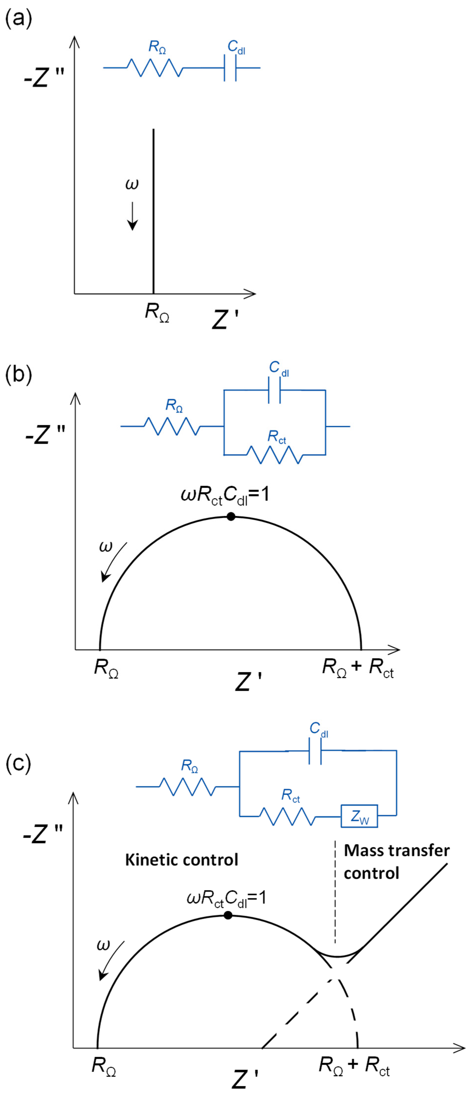 Figure 1. Complex plane impedance plots for selected electrical equivalent circuits: (a) capacitive interfacial response, (b) faradaic electron transfer reaction controlled by kinetics over the whole frequency range and (c) electron transfer reaction with mass transfer control at low frequencies. RΩ: cell resistance, Rct: electron transfer resistance, Cdl: double-layer capacitance, ZW: Warburg impedance.
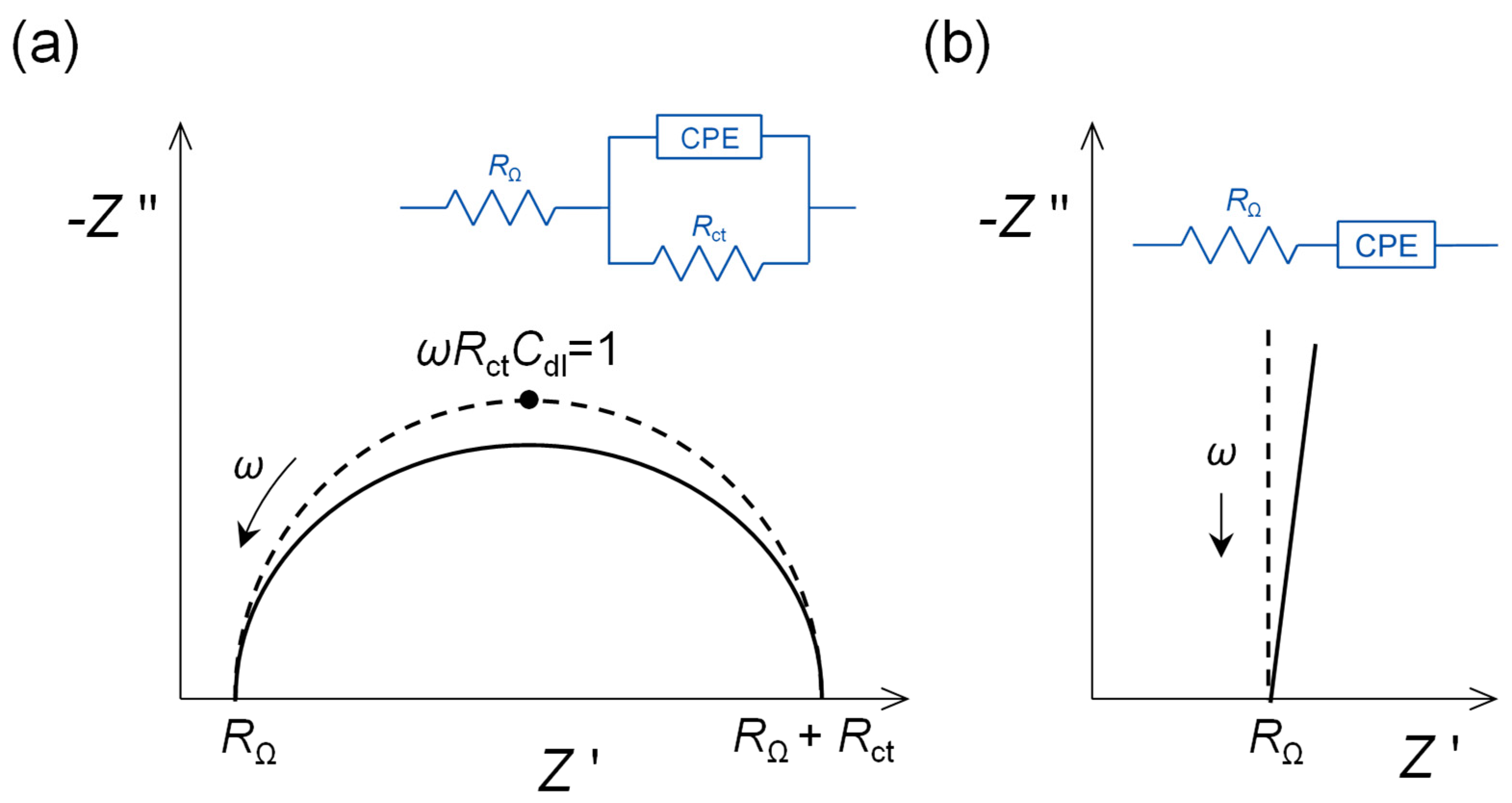 Figure 2. Complex plane impedance plots for selected electrical equivalent circuits with ideal capacitor response (dotted lines) replaced by non-ideal capacitor constant phase elements (CPE) (solid lines). (a) Faradaic electron transfer reaction controlled by kinetics over the whole frequency range, and (b) capacitive interfacial response.
A more complex example involves the spontaneous build-up of bilayers of myoglobin (Mb) and hyaluronic acid (HA) on a gold quartz crystal microbalance (AuQCM) electrode previously functionalised with sodium 3-mercapto-1-propanesulfonate (MPS) and poly (diallyldimethyl-ammonium chloride) (PDDA) [10]. Impedance spectra after the adsorption of each bilayer are shown in Figure 3a. The electrical equivalent circuit is the one shown in Figure 2a, but it is not immediately obvious what information can be deduced from the experimental spectra except for the values of R. Analysis of the capacitance, either ideal or non-ideal as a CPE, provides further information, taking each bilayer as having its own value of capacitance and summing the values of C−1 corresponding to capacitances in series. This analysis shows that for up to three bilayers, the capacitance values vary with each bilayer, but they become constant above three bilayers. Simple theoretical models employing constant bilayer capacitance values do not provide the correct profile, see Figure 3b. These deductions are corroborated by information from quartz crystal microbalance experiments and atomic force microscopy. Further details may be found in [10], and this illustrates the value of doing a full analysis of the spectra, and not just of R, which is common practice in many published articles.
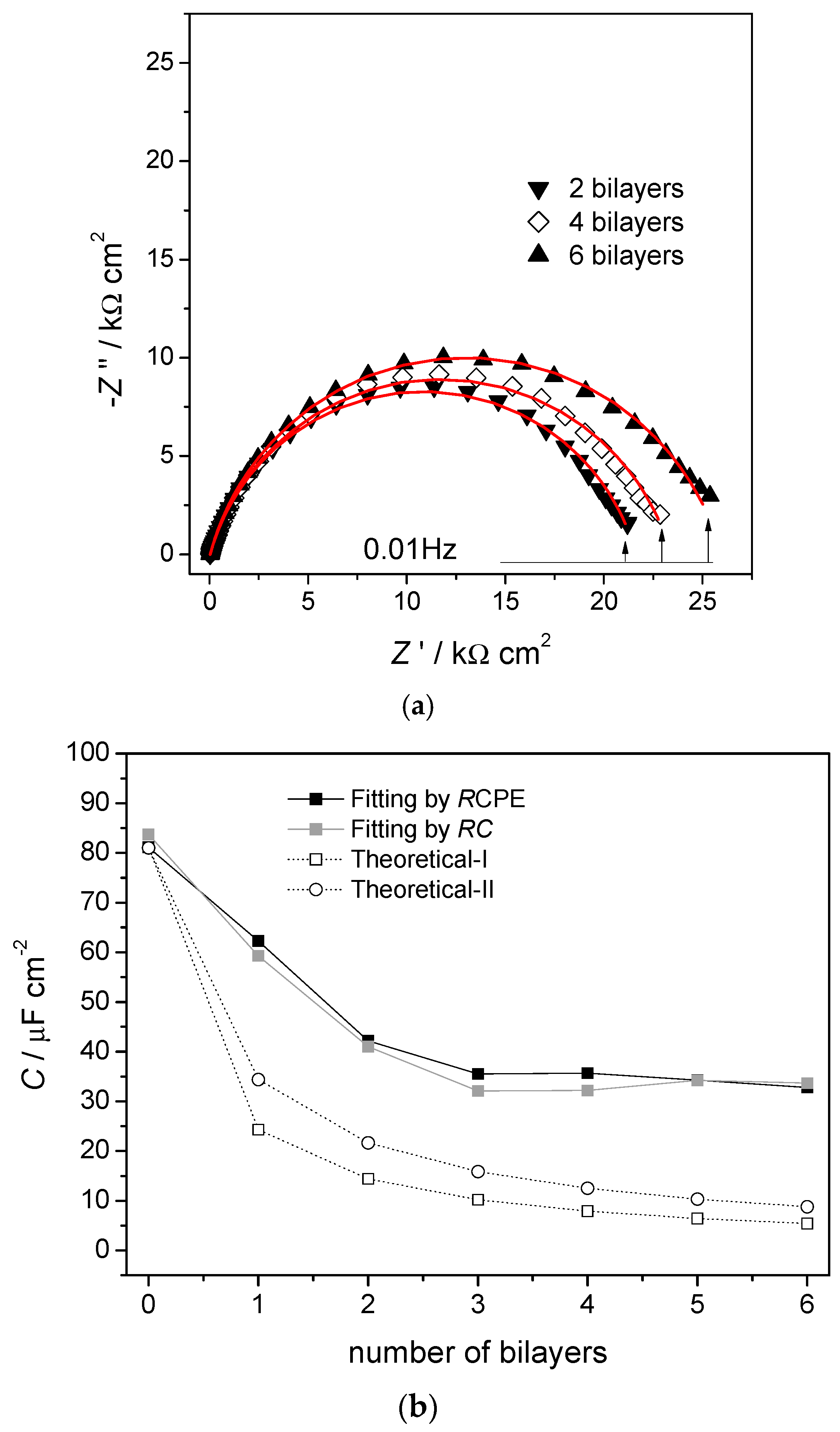 Figure 3. (a) Complex plane impedance plots recorded at gold quartz crystal microbalance (AuQCM)-modified electrodes in 0.05 M acetate +0.1 M KBr buffer solution, pH 5.0, at the OCP. (a) AuQCMMPS(−)/PDDA(+)/{HA/Mb}2–6, lines show equivalent circuit fitting to the circuit in Figure 2b. (b) Capacitance values. Dark squares, from RCPE equivalent circuit fitting to the experimental spectra; light squares, from RC semicircle modelling; (0) theoretical-I Ci = 34 μF cm−2 and (O) theoretical-II, Ci = 59 μF cm−2 obtained by summing contributions from successive bilayers. From [10], reprinted with the permission of the American Chemical Society, Washington, DC, USA.
2.2. Layer-by-Layer Modified Electrode Structures
Differences between layer-by-layer structures can be conveniently illustrated by recent papers that concern GCE modified by nanomaterials, without the addition of a redox probe.
First, GCE are modified with multiwalled carbon nanotubes (MWCNT) in chitosan, and then gold nanoparticles (AuNP) are deposited and they decorate the MWCNT, with the modified electrode finally being used to detect and quantify bisphenol-A (BPA) [11]. Impedance spectra can be recorded at different stages in the build-up process of the sensor and are shown in Figure 4 together with the equivalent electrical circuit used to model the spectra. The circuit includes two features, namely a high-frequency diffusion impedance representing diffusion through the modifier layers and a parallel RCPE combination to model the modified electrode–solution interface. For bare and AuNP-modified electrodes, it was not necessary to include the diffusion impedance for good fitting.
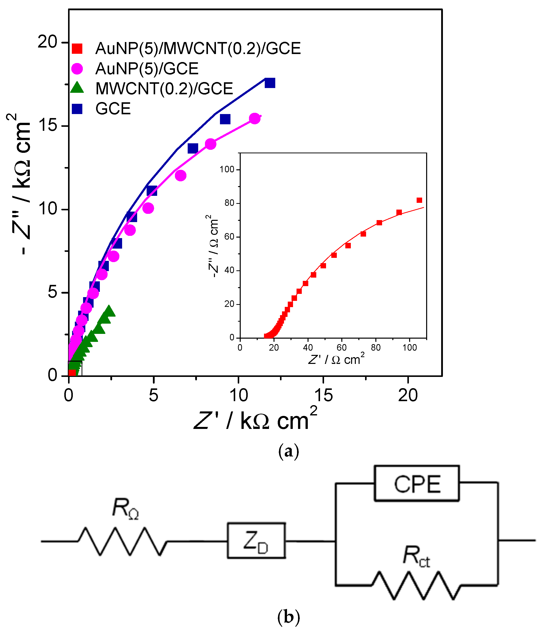 Figure 4. (a) Complex plane impedance plots at different electrodes in BR buffer (pH = 6) containing 9.0 mM BPA. Inset is the magnified plot of AuNP (5)/MWCNT (0.2)/GCE. Lines show equivalent circuit fitting. (b) Electrical equivalent circuit used to fit the spectra. From [11], reprinted with the permission of Elsevier, Amsterdam, The Netherlands.
The second illustration concerns electrodes modified with iron oxide nanoparticles (Fe2O3NP) in a chitosan dispersion (rather than MWCNT in chitosan), deposited on GCE [12]. On top of this, a polyphenazine redox polymer film is grown by potential cycling electropolymerisation. Three different polyphenazine films were grown in sulfuric acid-doped ethaline (choline chloride and ethylene glycol in a 1:2 ratio) deep eutectic solvent (DES). These were poly (neutral red) (PNR), poly (methylene green) (PMG) and poly (Nile blue) (PNB). The impedance spectra recorded afterwards in Britton–Robinson aqueous buffer solution showed the differences between the electrical characteristics of the three polymers, which can be ascribed to the different monomer structures. The variation with applied potential, another important variable, is similar for all three polymers. These impedance spectra show three features, each in a different frequency range. Apart from the two features shown in Figure 4 for electrodes modified with MWCNT and AuNP (that are diffusion impedance for diffusion through the modifier film in series with a parallel RCPE representing the electrode–solution interface), to model the spectra at very high frequencies, an additional parallel RCPE combination is needed, and that represents the interface between the electrode support and the modifier film, see Figure 5.
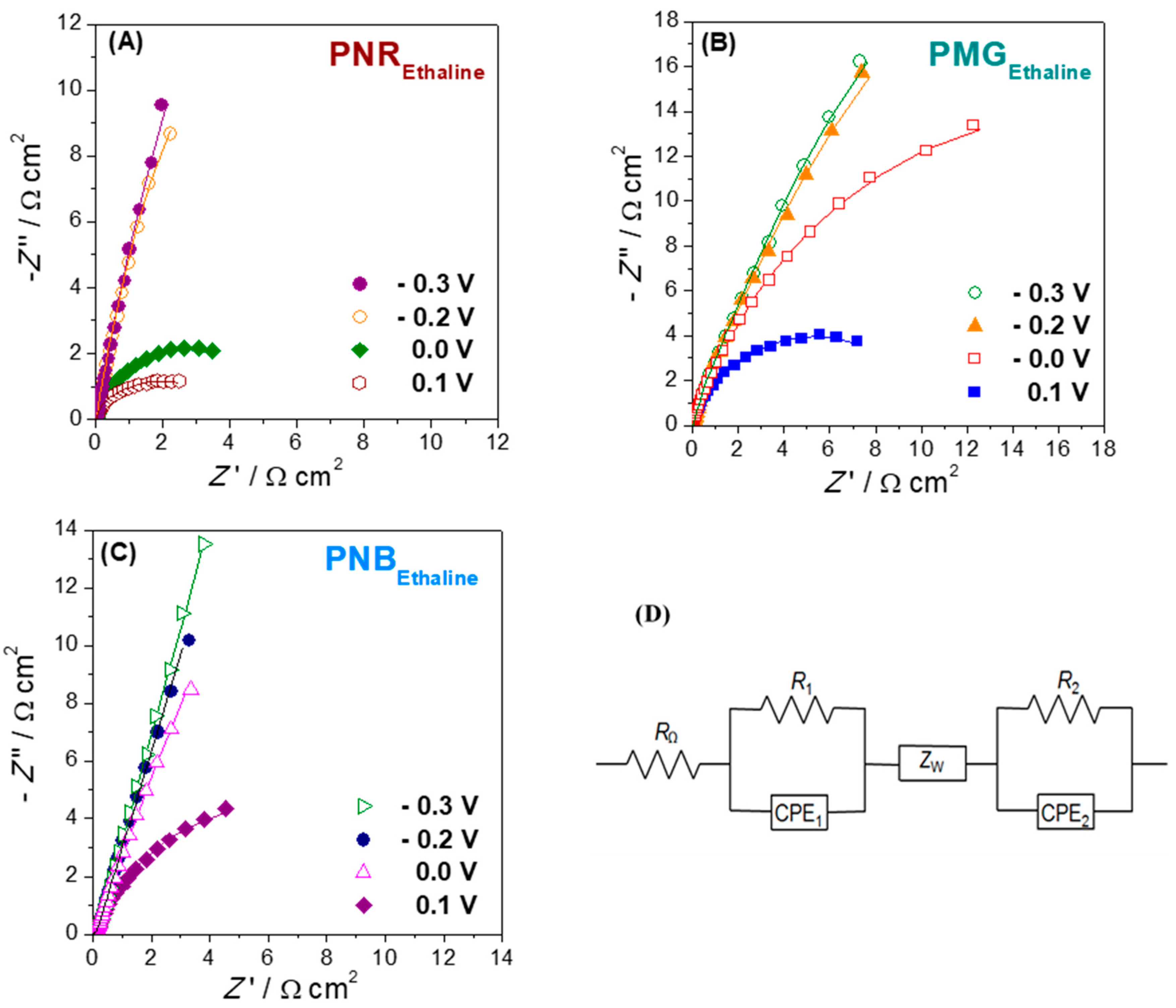 Figure 5. Complex plane impedance plots recorded in 0.1 M BR (pH 3.0) buffer solution at −0.3, −0.2, 0.0 and 0.1 V vs. Ag/AgCl at (A) PNREthaline/Fe2O3NP/GCE, (B) PMGEthaline/Fe2O3NP/GCE and (C) PNBEthaline/Fe2O3NP/GCE. (D) Electrical equivalent circuit used to fit the spectra. From [12], reprinted with the permission of Elsevier.
The general circuit shown in Figure 5 can be successfully used to model other cases involving nanomaterial-modified electrodes on which an electroactive redox polymer film is deposited.
An example in which the redox probe is used for characterisation during the build-up of the sensor is found in [13]. The redox probe is used to probe the effectiveness of immobilisation of successive elements of an immunosensor, although the quantification itself is performed by cyclic voltammetry, obtaining a detection limit of 0.8 ng/mL for carcinoembryonic antigen detection. Other examples are described in [14], in the assembly of aptasensors with carbon nanomaterials. Aptamers are DNA-derived oligonucleotides and an alternative to native antibodies and can be tuned more easily to the structure of specific analyte species.
This entry is adapted from the peer-reviewed paper 10.3390/molecules27051497
This entry is offline, you can click here to edit this entry!