The path from molecular to meteorological scales begins with the persistence of molecular velocity after collision inducing symmetry breaking, from continuous translational to scale invariant, associated with the emergence of hydrodynamic behaviour in a Maxwellian (randomised) population undergoing an anisotropic flux. The statistical multifractal formulation of observed atmospheric variability enables the examination of turbulence. The unexpected correlation between the intermittency of temperature and the ozone photodissociation rate in the lower Arctic stratosphere led to an analysis of the role of Gibbs free energy in the general circulation of the atmosphere, and a suggestion to solve the persistent cold bias in its siumlation by free running numerical models.
1. Microscopic and Macroscopic Processes
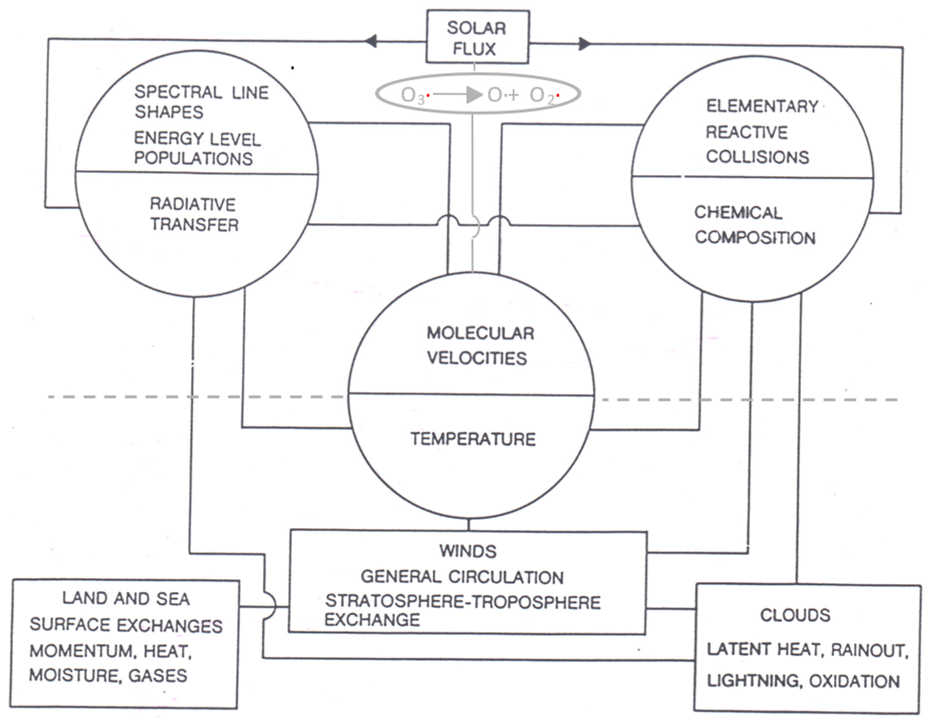
The coupling of molecular and meteorological processes is shown schematically in Figure 1. It is through the central variable of temperature.
Figure 1. The determination of measured temperatures by molecular velocities is how microscopic processes couple to meteorological ones. The observed correlation between the ozone photodissociation rate and the intermittency of temperature was an indication that local thermodynamic equilibrium in lower stratospheric air was not a valid assumption. Note that aerosols, not shown, play a significant role in chemical composition, cloud physics and radiative transfer. The Gibbs free energy resulting from the difference between the incoming low entropy beam of solar flux (high energy UV and visible photons) and the outgoing higher entropy terrestrial flux (low energy infrared photons) over the entire 4π solid angle provides the work necessary to drive the circulation. The scales can be specified approximately as micro: 10−10 to 10−8 m, meso: 10−8 m to 10−6 m, macro: >10−6 m. One micron, 10−6 m, is approximately the largest size of aerosol which can remain suspended in the troposphere and be transported significant distances by the winds.
1.1. Persistence of Molecular Velocity after Collision
The persistence of molecular velocity after collision
[1] breaks the continuous translational symmetry (randomness) assumed in speed and direction that underlies the Maxwell–Boltzmann probability distribution function (PDF) and hence Lorentzian and Doppler spectral line shapes used in radiative transfer in the atmosphere. Einstein–Smoluchowski diffusion is also negated in the atmosphere and with it the definition of temperature used in laboratories. Maxwell–Boltzmann PDFs have continuous translational symmetry, which is broken by the persistence of velocity after collision.
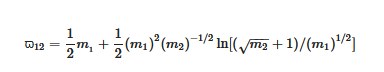
The persistence ratio ϖ12 is the ratio of the mean velocity after collision to that before collision between molecules of masses m1 and m2. If m1 = m2 then ϖ12 = 0.406, but in general for m1 ≠ m2 the heavier molecule will be slowed less than the lighter one.
This breaking of continuous translational symmetry will be discussed further later in the light of observational analyses, but it immediately leads to the interpretation of molecular dynamics calculations that showed the emergence of hydrodynamic behaviour in a population of randomised molecules subject to an anisotropic molecular flux
[2]. This phenomenon is shown in
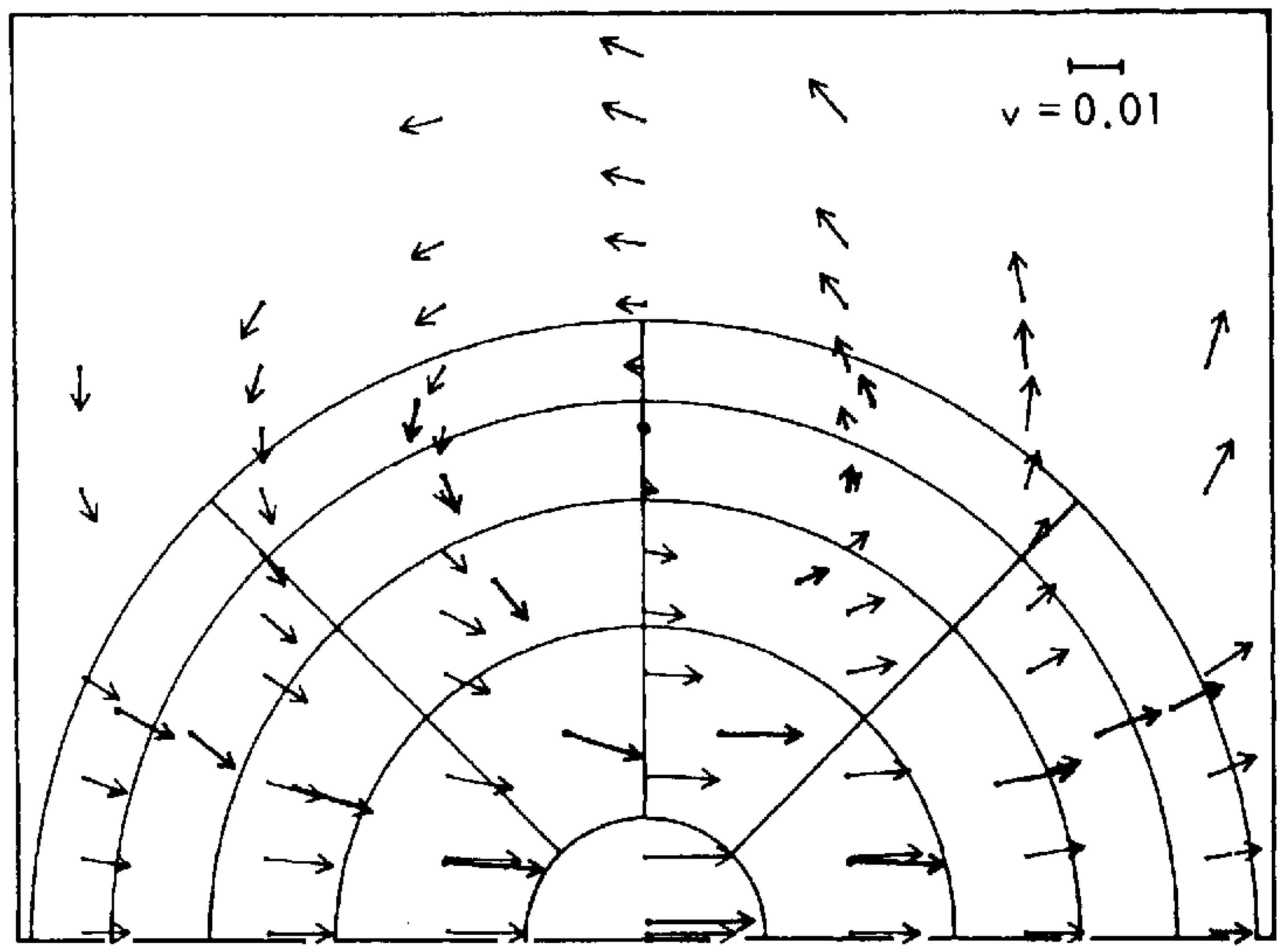
Figure 2. Here ‘molecules’ are represented as hard spheres (‘billiard balls’); ring currents—vortices—emerged on very short time and space scales.
Figure 2. The original simulation of the emergence of ‘ring currents’—vortices—in a population of Maxwellian atoms subject to an anisotropic flux
[2]. The thicker arrows represent averages over the molecular velocity vectors after 9.9 collision times, whereas the thinner arrows represent simulation by the Navier–Stokes equation. Later simulations showed disagreements between the two approaches.
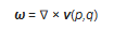
It is suggested from the outset that a vorticity approach be adopted from this smallest, molecular scale. Let
ω be the vorticity of the field of molecular velocity
v [3]:
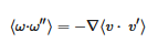
This enables calculation of twice the enstrophy directly by taking the curl of the molecular velocity field
Because enstrophy propagates downscale, in 2D theory at least, it may be less suited to describing the behaviour of energy deposited on the smallest scales, that of photons and molecules as it is in the atmosphere. The vorticity correlation function can lead to the vorticity form of the Navier–Stokes equation; see Section 3.3 of
[4]. Nevertheless, the vorticity of ‘air’ in a molecular dynamical calculation is obtainable by:
where
p is molecular momentum and
q is molecular position. They are necessitated by the non-spherical symmetries of real molecules and the omnipresent anisotropies of gravity, planetary rotation and the solar beam. The
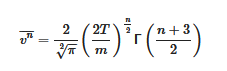
nth moment of the molecular speed is
[3][4][5]:
This equation permits n to be used in calculating moments in the course of statistical multifractal analysis of molecular dynamics calculations.
1.2. Emergence of Fluid Flow from a Molecular Population
Figure 2 illustrates the discovery of this phenomenon by Alder and Wainwright
[2]. It was appealed to in a meteorological context as the result of an unexpected observational correlation between the ozone photodissociation rate and the intermittency of temperature
[3], about which more later. Physically, the mechanism consists of the faster molecules pushing up higher number density ahead of themselves, leaving lower number densities in their rear. The resulting number density gradient results in a flux of the more numerous, nearly average molecules that produces the ring current. The numerous, near average molecules exchange collisional energy easily, and in so doing maintain an operational temperature, which is not, however, described by a Boltzmann PDF. Note that the interactions are non-linear and result in the vorticity structure being self-sustaining, offering the ability to propagate upscale.
Extant statistical multifractal analyses expected temperature to scale like a passive scalar (a tracer), but the earliest such treatments of NASA ER-2 data in the lower stratosphere at 17–20 km altitude showed that temperature scaled differently than known tracers
[6][7][8], at least under rescaled range analysis. With the availability of high-resolution GPS dropsonde data from the NOAA Gulfstream G4-SP, it became clear from statistical multifractal analyses that temperature was affected differently by gravity than other variables
[4][9][10][11]. The scaling of temperature spans the range from micro (molecular) through meso (nanometres to micrometres) to macro (>micrometres). That accounts for temperature acting as a kind of integrator in the way that other variables do not.
A further implication of the Alder–Wainwright mechanism is in the basis of the fluctuation–dissipation theorem as embodied in the Langevin equation. Langevin treated the mean as organised behaviour and fluctuations as dissipation. The Alder–Wainwright mechanism implies the reverse, that the hydrodynamic fluctuation carried by the fastest molecules represents emergent organisation and the mean represented by the near average molecules represents dissipation that defines an effective temperature.
We cannot expect to view atmospheric vorticity in two dimensions and remain quantitative, because the dimensionality of atmospheric flow is 2 +
H(s),
[12][13][4] where
H(
s) is the vertical scaling exponent of the horizontal wind,
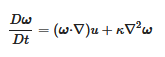
s. The vorticity form of the Navier–Stokes equation is:
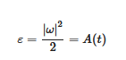
where κ is kinematic viscosity. The first term on the right says that vorticity, ω, advects itself: nonlinearity is inherent. This term alone is responsible for much of the complexity and difficulty associated with understanding, describing and computing atmospheric flow. ω is defined by Equations (2) and (3) and using (3) we can relate the autocorrelation function for vorticity, A(t), to the enstrophy ε:
Enstrophy is governed by:
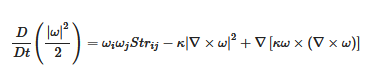
where Strij is the straining rate on a fluid element.
Equation (8) expresses the generation of vorticity by stretching, or its destruction by compression, via the first term, balanced by viscous dissipation in the second term. The third term is the divergence, often assumed to be locally zero; this cannot be strictly true, for example, if ozone photodissociation is leading to the generation of vorticity. Considering the theoretical case of 2D turbulence, there are reverse cascades of energy and enstrophy, upscale for the former and downscale for the latter. If photon energy is directly converted to vorticity as implied by the Alder–Wainwright mechanism, it would imply energy transfer upscale from the smallest, molecular, ones in the range of 10–100 nanometres at tropospheric temperatures and pressures. However, the point is moot because the scale invariant structure of the fluctuating abundances of the absorbers and emitters of radiation, including ozone, carbon dioxide, methane, nitrous oxide, halocarbons, aerosols and water in all its phases, means that energy is input and lost to air on all scales, eliminating the possibility of conservative energy or enstrophy cascades either upscale or downscale. The observed scale invariant 23/9 dimensionality of air also eliminates 2D theories from relevance.
2. Statistical Multifractality
The variability in air is defined by three multifractal scaling exponents, which have been evaluated from observations of adequate quality
[14][15][16][17]. The mathematical structure underlying the definition of
H, C1 and
α may be found in these references; the notation is that in
[15][16].
Table 1 shows equivalences between the variables of equilibrium statistical thermodynamics and the scaling variables from statistical multifractal analysis as applied to open, non-equilibrium systems, which the atmosphere is. The equivalences in
Table 1 result from mappings
[14] via Legendre transforms; they are not merely formal similarities and lead to the thermodynamic form of multifractality
[16].
Table 1. Equivalence between statistical thermodynamic and scaling variables.
| Variable |
Statistical Thermodynamics |
Scaling Equivalent |
| Temperature |
T |
1/qkBoltzmann |
| Partition function |
f |
e−K(q) |
| Energy |
E |
γ |
| Entropy |
−S(E) |
c(γ) |
| Gibbs free energy |
−G |
K(q)/q |
The variables are obtained as follows. q defines the qth order structure function of the observed quantity. The scaling exponent K(q) is derived from the slope of a log–log plot of the signal fluctuations versus its range, and H is obtained from:
and examination of energy E in terms of a scale ratio produces an expression for the fractal co-dimension c(γ). C1 is the co-dimension of the mean, characterising the intensity of the intermittency. The Lévy exponent α characterises the generator of the intermittency which is the logarithm of the turbulent flux; for a real system, its value may not be confined to the theoretical range.
In practice here we find
H = 0.56,
C1 = 0.05 and
α = 1.60. The theoretical ranges are 0 <
H < 1; 0 <
C1 < 1 and 0 <
α < 2. A Gaussian has
H = 0.50,
C1 = 0 and
α = 2. See
[4][15][16] for further discussion, and below for analysis of observations. The actual values of the three scaling exponents for wind, temperature, ozone and other molecules may provide information about the variables and how they interact.
2.1. Vertical Scaling: Horizontal Wind, Temperature and Humidity
Figure 3 summarises the 2006 data
[11].
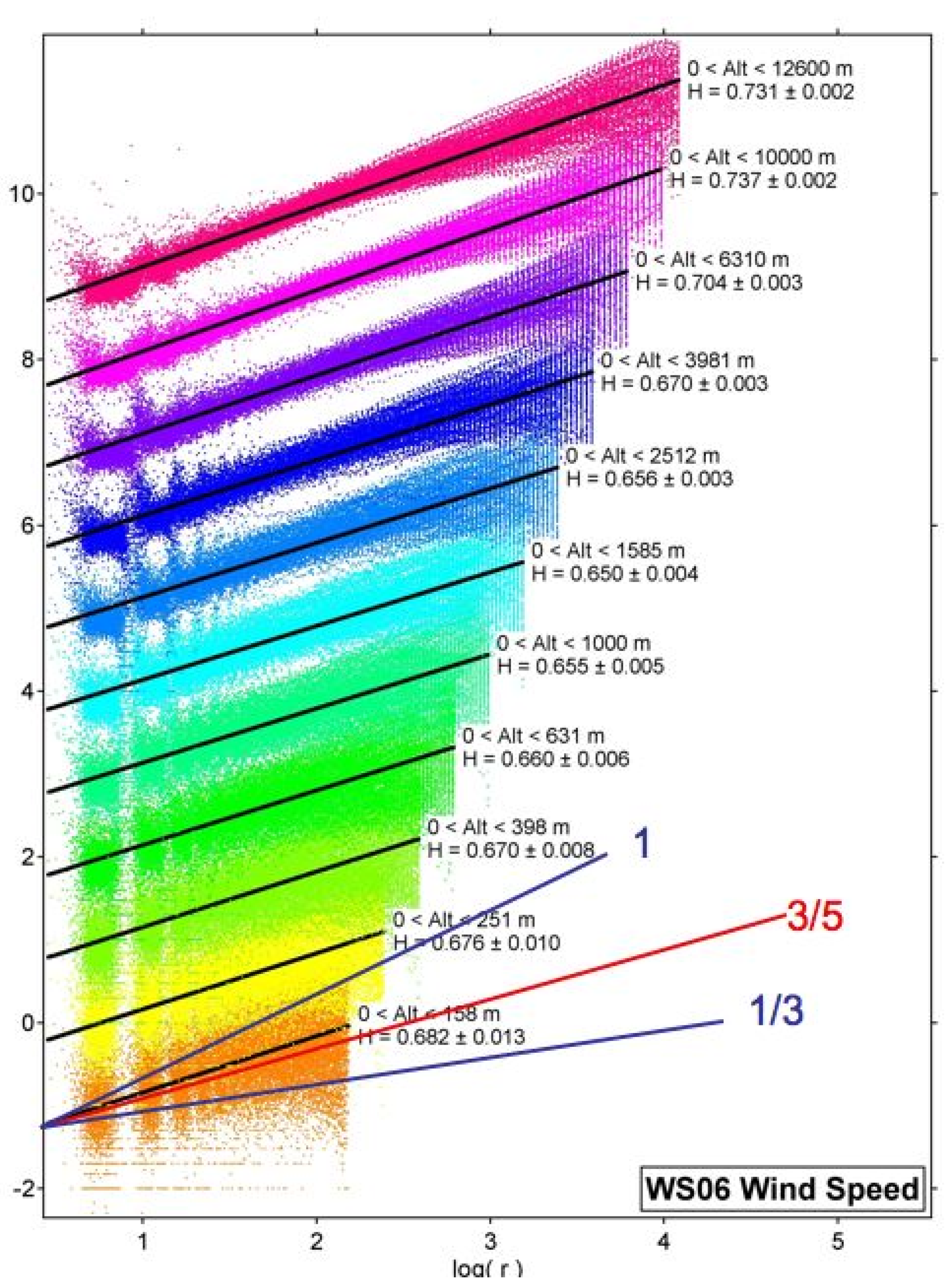
Figure 3. H is the vertical scaling exponent of the horizontal wind observed by 315 GPS dropsondes from the NOAA G4-SP aircraft flying at an altitude of about 13 km in January–March 2006 in the area bounded by (21°–60° N, 128°–172° W). Each coloured set of points represents H and the black lines are the root mean square fits to the vertical shear across layers, increasing logarithmically upwards and labelled by the corresponding value of H. The three lines labelled by fractions are what different theories predict. Gravity waves 1, Bolgiano–Obukhov 3/5, Kolmogorov 1/3. H increases to near 0.75 at 12 km, where jet streams were prevalent. Isotropy (Kolmogorov) is nowhere evident.
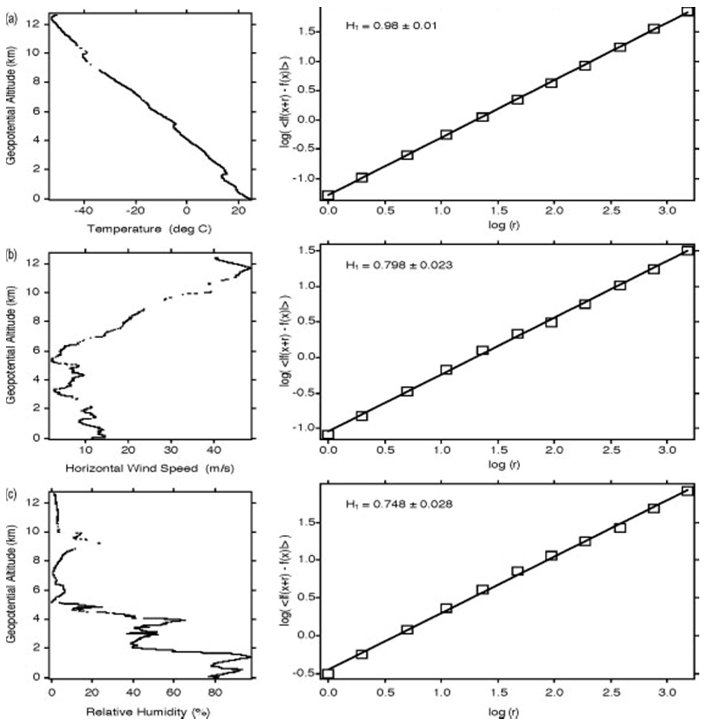
If the vertical scaling of temperature is calculated via spectral analysis, assuming for the purpose that intermittency is negligible, the value of
H is approximately 5/4 while
H for wind speed and relative humidity remains unchanged from the values in
Figure 4b,c, respectively. The different scaling for temperature has been attributed to the effect of gravity on air density, upon which it acts directly, unlike wind speed and relative humidity
[18]. It will be seen later that the effects of scaling in jet streams are also significant.
Figure 4. The descent from 13 km at (15°15’11″ N, 165°59′42″ W) on 20040229. The two frames in each of (
a–
c) show the profile and variogram for temperature, wind speed and relative humidity respectively.
H is calculated from the slope of the variogram. Note that temperature scales differently than wind speed and humidity
[11][18]; the temperature profile is smoother than those for wind speed and relative humidity, reflected in the value of
H approaching 1.
The dropsonde results are also apparent in stability analyses of all drops treated fractally
[10]. The results were valid for dry adiabatic, dynamic (Richardson number) and moist adiabatic approaches. The correlation co-dimensions were respectively 0.36, 0.22 and 0.15, a demonstration of the importance of wind shear and moisture compared to a static dry adiabatic analysis. The corresponding fractal dimensions of the Cantoresque set are 0.64, 0.78 and 0.85.
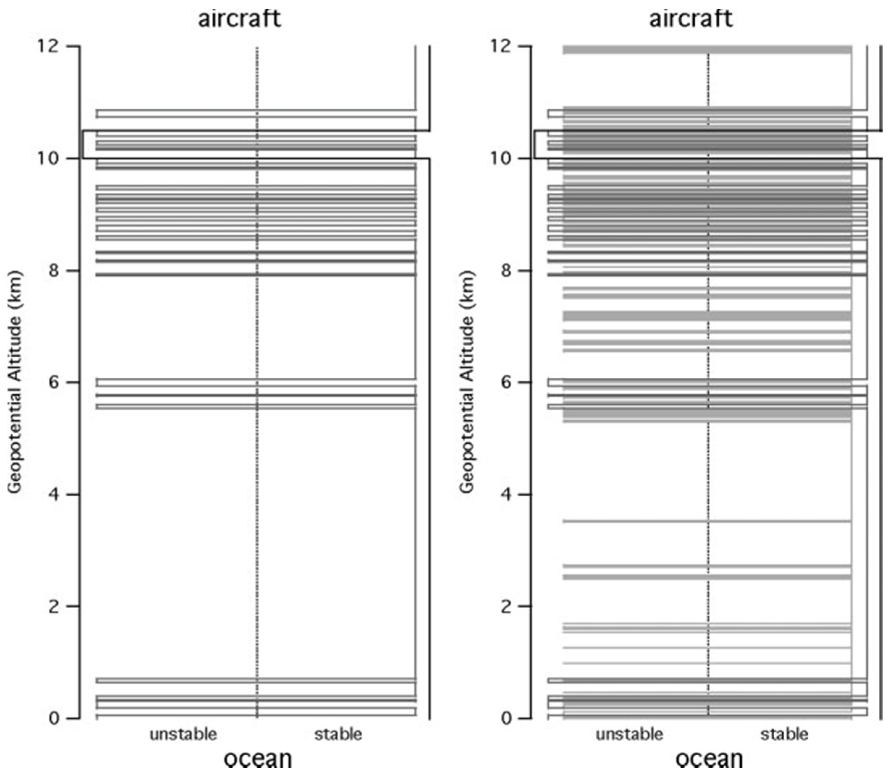
In
Figure 5, for one descent at 500 and 50 m resolutions, a broadly unstable lower troposphere and stable upper troposphere is seen, whereas at 15 m there are embedded unstable layers within stable layers at all scales, forming a ‘Russian doll’ structure characterised by a fractal dimension of 0.65. There are no unstable layers below about 50 m vertical dimension. This sonde was one of a pair dropped simultaneously; the high correlation of the structures seen by the two sondes eliminates the possibility that the signal is generated by noise
[10].
Figure 5. The stability of the atmosphere derived from a GPS dropsonde descent from the NOAA G4-SP aircraft at 13 km at (25° N, 157° W) on 20040229, using the criterion Ri > 1/4. The unstable layers are to the left, the stable ones to the right, with horizontal lines marking the transitions between the layers. The left-hand diagram shows the transitions at 500 m and 50 m resolutions. The right-hand diagram shows the results at 500, 50 and 15 m.
Composite variograms from all 246 useable dropsondes during the Winter Storms 2004 mission, involving 10 flights over a wide area of the eastern Pacific Ocean of the Northern Hemisphere
[11], are shown in
Figure 6. See
[4][10][11] for further description and analysis.
Figure 6. The composite variograms for the 2004 Winter Storms mission. (a) temperature, (b) wind speed, (c) relative humidity. Although wind speed and relative humidity have H values of about 0.75, the temperature has values of slightly less than unity, which can be expected from the smoothness of the vertical profile typified in Figure 4a compared to the rougher curves for wind speed and relative humidity in Figure 4b, c. If for the purpose intermittency is ignored, spectral analysis yields about 1.25 for temperature but leaves the values for wind speed and relative humidity unchanged.
The ‘horizontal’ scaling of the aircraft observations has been calculated separately for the NASA ER-2 and WB57F mainly in the lower stratosphere, and for the NOAA G4-SP and NASA DC-8 mainly in the upper troposphere
[4]. We note that there is an element of vertical velocity in such flight segments
[19], and that during their ‘vertical’ segments the results for temperature, wind speed and humidity for the scaling exponent
H agreed within 10% with the dropsonde results in the previous section
[4][11]. The missions concerned ranged from pole to pole
[4][11][20] when the DC-8 is included.
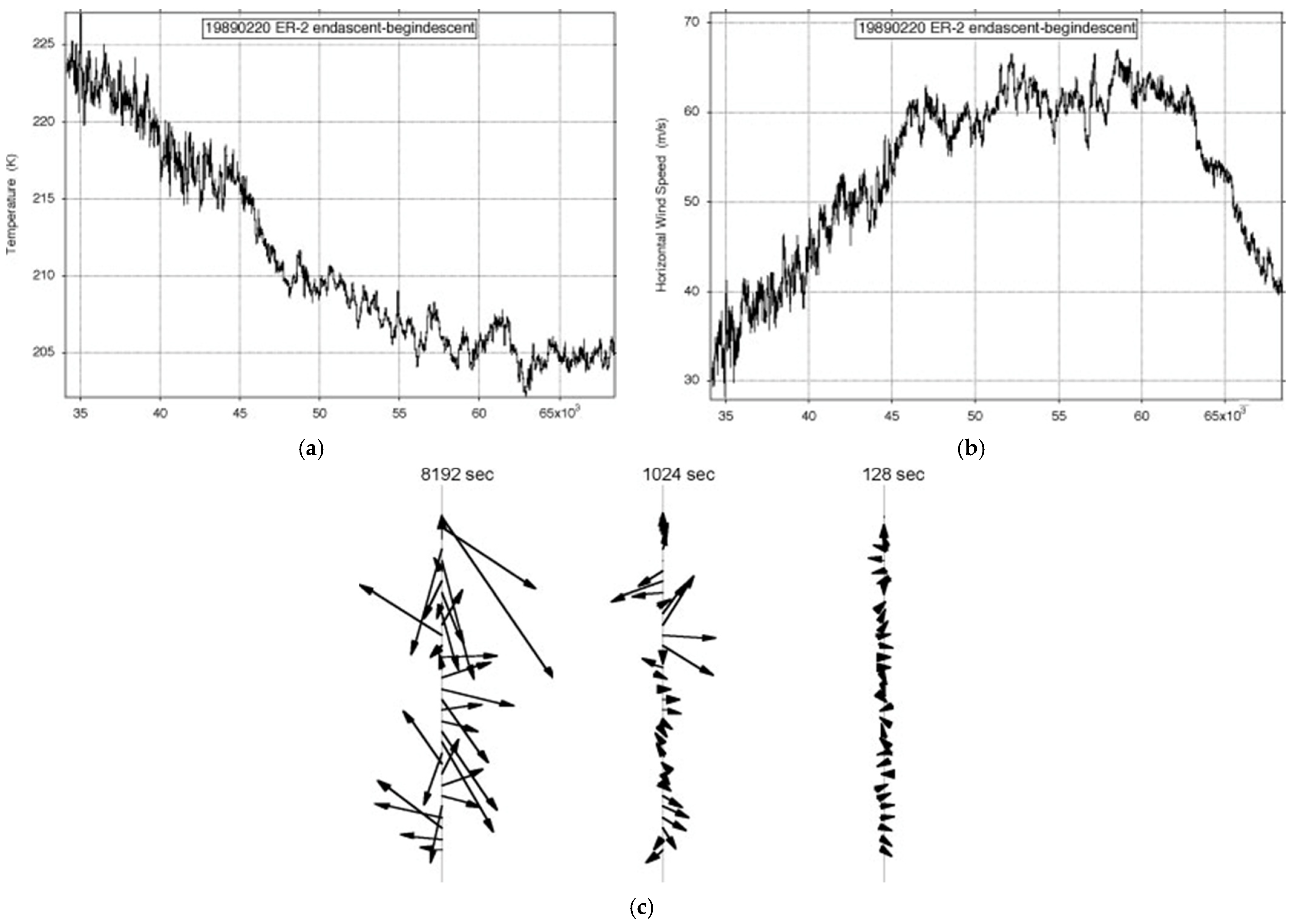
Figure 7 shows the observations of the longest ER-2 flight available, just over an Earth radius long on 19890220. It was one of the few on Arctic missions AASE, AASE-II and SOLVE that was along rather than across the lower stratospheric polar night jet stream (SPNJ). There were none along the Antarctic SPNJ during AAOE and ASHOE-MAESA
[4][20]. There was a greater incidence of more variable encounters with jet streams by the WB57F during WAM, ACCENT, pre-AVE and CRYSTAL-FACE and by the G4-SP during Winter Storms 2004–2006, with the subtropical jet stream (STJ) and the polar front jet stream (PFJ); see
[21].
Figure 7. ER-2 flight from (59° N, 6° E) to (38° N, 75° W) on 19890220: (a) temperature, (b) wind speed, (c) shear vectors averaged over intervals differing by a factor of 23. The length of the flight exceeded an Earth radius; the aeroplane flew at 200 ms−1.
2.2. Scaling in Jet Streams
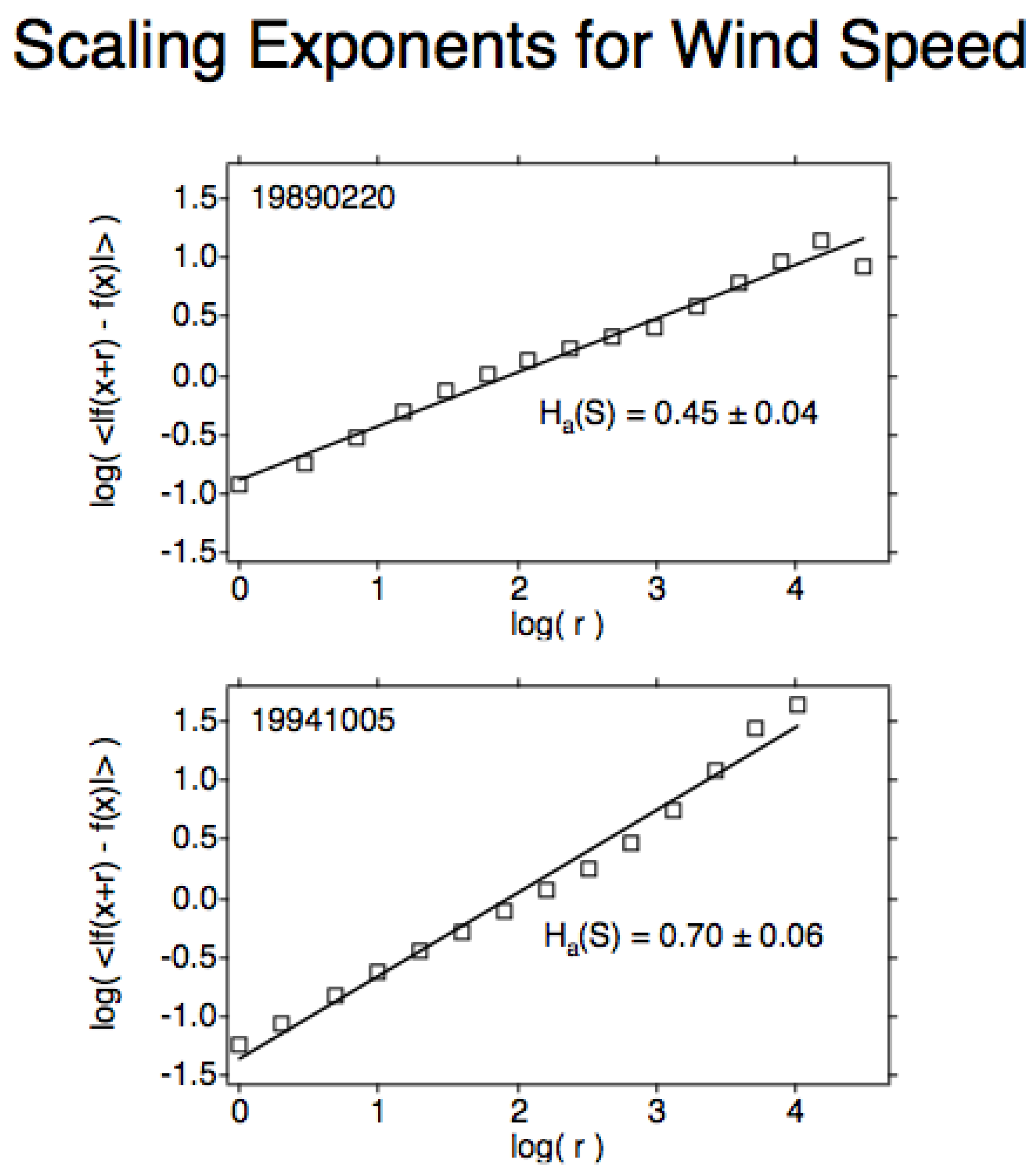
Figure 8 shows the scaling exponent
H for wind speed during ER-2 flight segments along the Arctic SPNJ and across it for the Antarctic SPNJ. The result that the along jet flight segment has the lowest value of
H for wind speed suggests that this most highly anticorrelated value is caused by the speed shear being more effective at producing less organised, more random flow than is directional shear. The directional shear then probably accounts for the higher value in the across-jet direction, corresponding to stronger, more organised flow. The results are consistent with the shears in
Figure 7c and are responsible for the exchange of air and its chemical content between the vortex and its surroundings
[4][15][22].
Figure 8. (Upper), the scaling exponent H for wind speed along the Arctic SPNJ; 0.45 is the lowest value recorded on all 140 qualifying ER-2 flight segments. (Lower), the value of H for wind speed across the Antarctic SPNJ; 0.70 is the highest value recorded on the 140 flight segments.
2.3. Molecular and Photochemical Effects
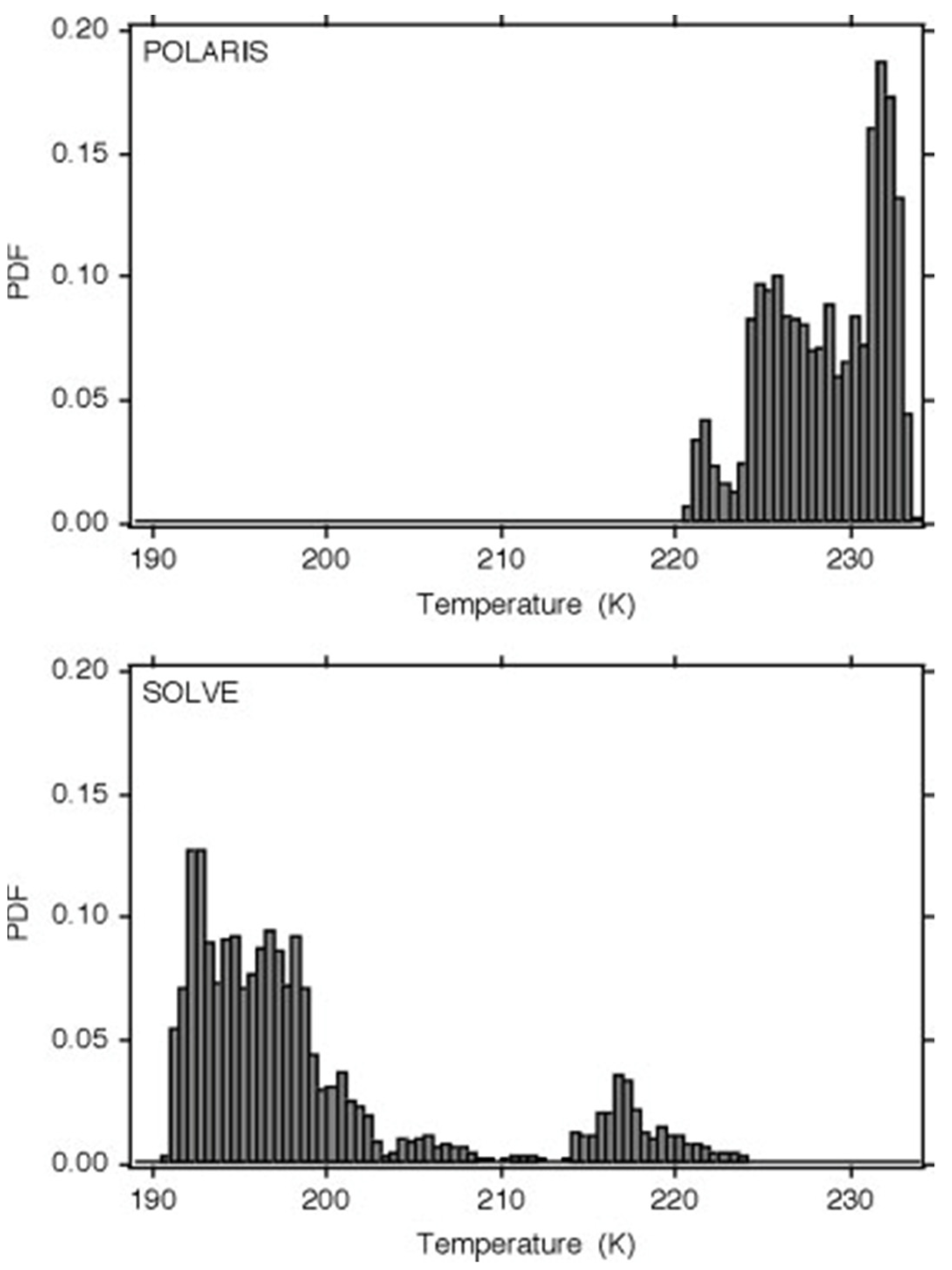
The intimate connection between molecular behaviour and temperature seen earlier necessitates further examination of the behaviour of temperature in terms of its PDF, intermittency and the correlation of the latter with the ozone photodissociation rate. The observations were taken in the lower stratosphere during Arctic summer (April–September) in 1997 (POLARIS) and Arctic winter (January–March) in 2000 (SOLVE).
Figure 9 shows the highly non-Gaussian PDFs. These missions had measurements of the ozone photodissociation rate
[23] and are discussed in
[3][4] and in the next section.
Figure 9. Probability distribution functions of temperature from Arctic summer 1997 (upper) and Arctic winter (lower). There are millions of 1 Hz points, taken between 18 and 20 km from the ER-2 flying at 200 ms−1. In summer there is a warm most probable value with a fat cool tail, and in winter a cool most probable value with a fat warm tail. The distributions are highly non-Gaussian.
The relation between temperature and molecular velocity is given by equations 3.1 and 5.1 of
[4]:
3. The Intermittency of Temperature and Its Correlation with Ozone Photodissociation Rate
An unexpected result from the measurement [23] of the ozone photodissociation rate, J[O3], was positive correlation with the intermittency of temperature, C1(T). That triggered a search for an explanation, with the causal attribution being the production of translationally hot O and O2 photofragments recoiling into and acting in the vortices produced by the mechanisms seen in Figure 1 and justified in references [3][4][24]. The results from POLARIS in the Arctic summer of 1997 and from SOLVE in the Arctic winter of 2000 are displayed in Figure 10. C1 (T) is positively correlated both with the ozone photodissociation rate and with temperature itself. By viewing Figure 9 in conjunction with Figure 10 and Figure 11, it can conclude that atmospheric temperature is not that of a gas in local thermodynamic equilibrium [18][25]. Account must be taken of molecular behaviour from the smallest scales up to the gravest; it will mean acting on the persistence of molecular velocity after collision [1] and its breaking of continuous translational symmetry of a thermalised gas via the Alder–Wainwright mechanism [2].
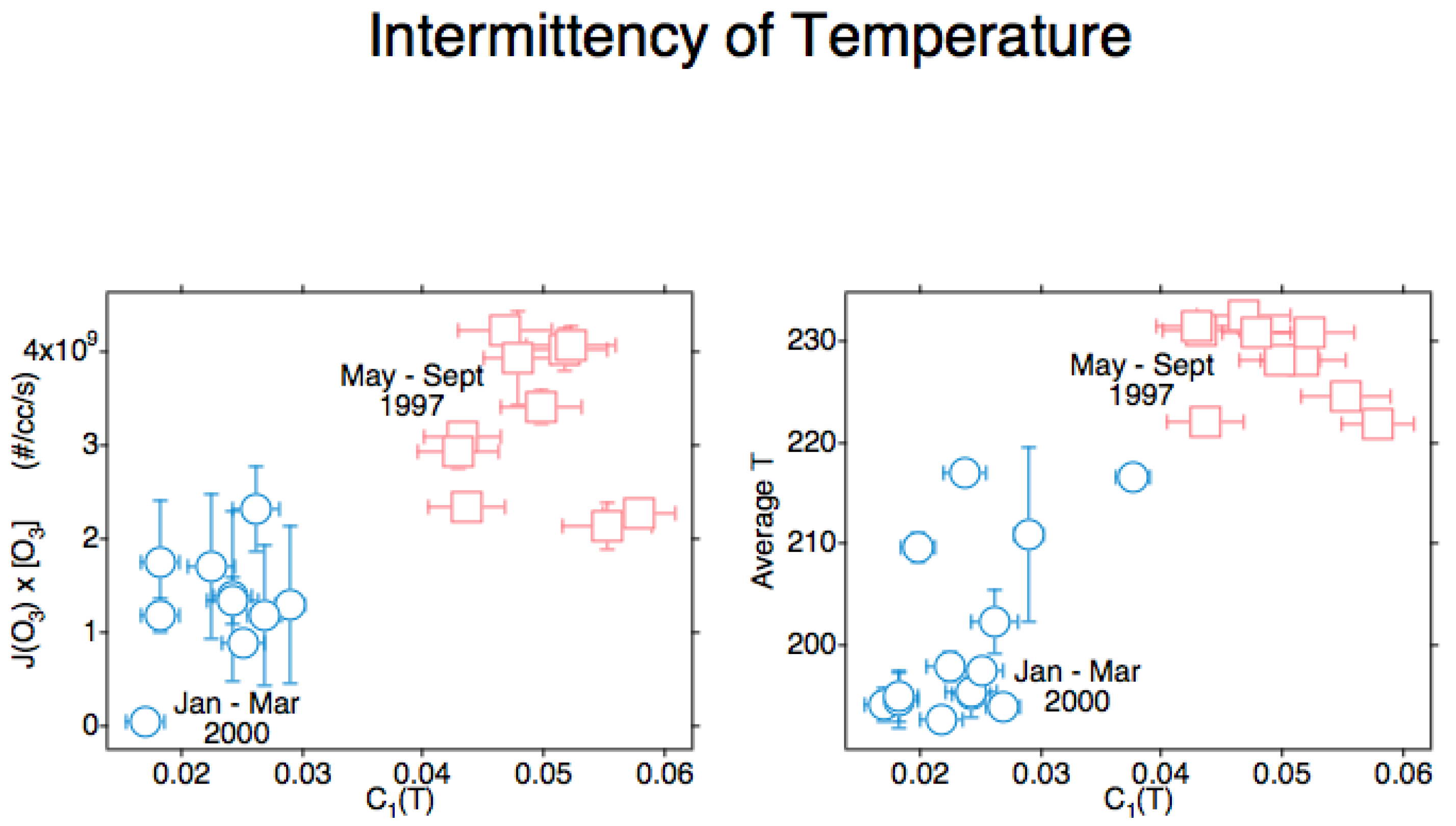
Figure 10. These Arctic data are from all suitable ER-2 flights in April–September 1997 and January–March 2000. The ozone photodissociation rate J(O3)[O3] is averaged over the flight segment, the vertical bars indicating the standard deviation in the left diagram with the intermittency of temperature on both abscissae. In the right diagram, the temperature on the ordinate is averaged over the flight segment, with the vertical bars indicating the standard deviation. In both diagrams, the intermittency exponent C1 for temperature T is obtained from the slope of the curve as shown in the lower right diagram of Figure 17. Both ozone photodissociation rate and temperature itself show positive correlation with the intermittency of temperature as measured from the aeroplane; these are respectively cause and effect.
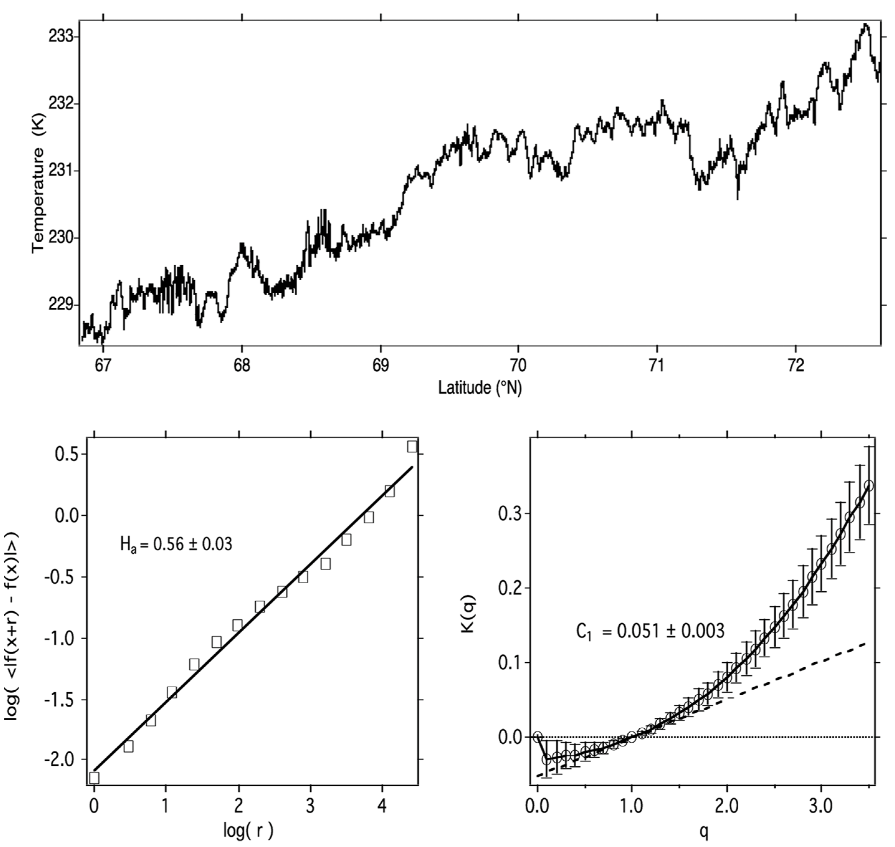
Figure 11. (
Upper) Temperature along ER-2 flight segment in the summer lower Arctic stratosphere, 19970506 (yyyymmdd). (
Lower left) The log–log plot used to derive the
H scaling exponent. (
Lower right) Plot used to derive the graph of
K(q) vs.
q from which
Figure 18 was calculated. See Table 1 and Figure 1 of
[16].
5. Scaling Based Entropy and Gibbs Free Energy
Given that the airborne in situ measurements of molecular species and photodissociation rates are unlikely to become routine, and are presently unattainable from satellite remote sounding, what can be done? Either locally by airborne methods or globally by satellites, it is not foreseeable to the extent necessary. One alternative approach is outlined in
[16], where the thermodynamic form of statistical multifractality
[14] is adapted
[16] to produce
Table 1. Those results enable diagnosis of steady states and system directionality from winds and temperatures, which are observed globally in a routine manner. The results in
[16] vindicate the ‘bare’ cascade models of Schertzer and Lovejoy
[13] and Lovejoy and Schertzer
[14] by producing results from ‘dressed’ curves such as that in
Figure 12, based on the data in
Figure 11. Similar results were obtained for wind speed and ozone and are representative of all suitable 140 ER-2 flight segments between 1987 and 2000. Here, it is suggested that these diagnostics should prove applicable to global atmospheric models, particularly those dealing with air pollution and climate, wherein molecular species have to be simulated. Gibbs free energy does the work that drives the circulation to a different steady state under a perturbation, either on cooling or heating, after the entropic effects of dissipation have been accounted for.
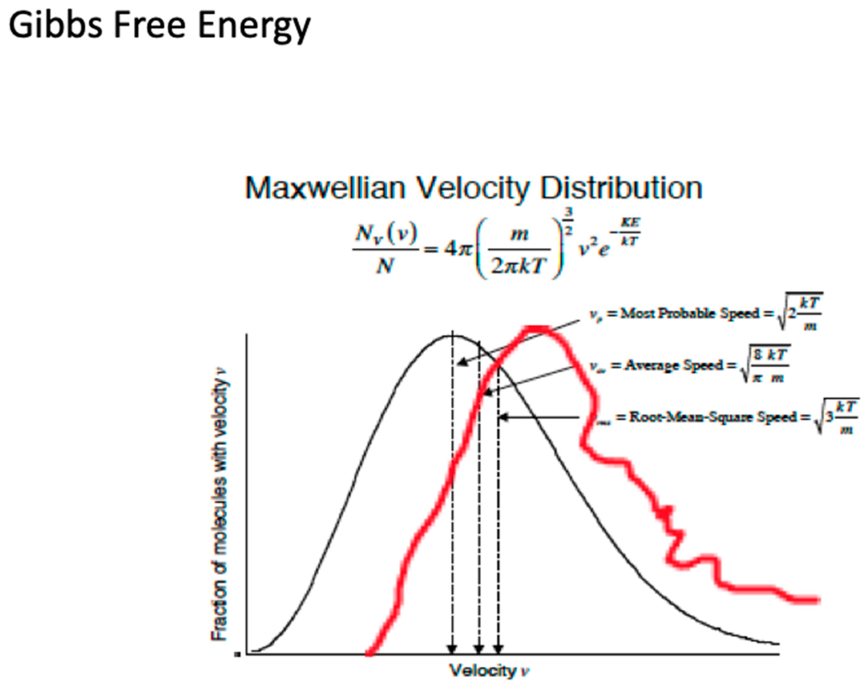
What molecular behaviour should be expected in the nonequilibrium conditions displayed in Figure 11 and Figure 12? How will translationally hot and rotationally hot air molecules be manifest, whether observed by, for example, direct molecular beam sampling instruments or calculated by molecular dynamics methods? The red curve in Figure 13 is a hypothetical curve of the PDF of such molecular velocities, whereas the black curve represents an equilibrium Maxwell–Boltzmann state. The difference of the integrals beneath them via Equation (10) provides the Gibbs free energy. The atomic and molecular fragments from ozone photodissociation, which happens from the ultraviolet Hartley band through the Huggins, Chappuis and Wulf bands that stretch across the visible to the near infrared, can have up to an order of magnitude more energy than the average molecules.
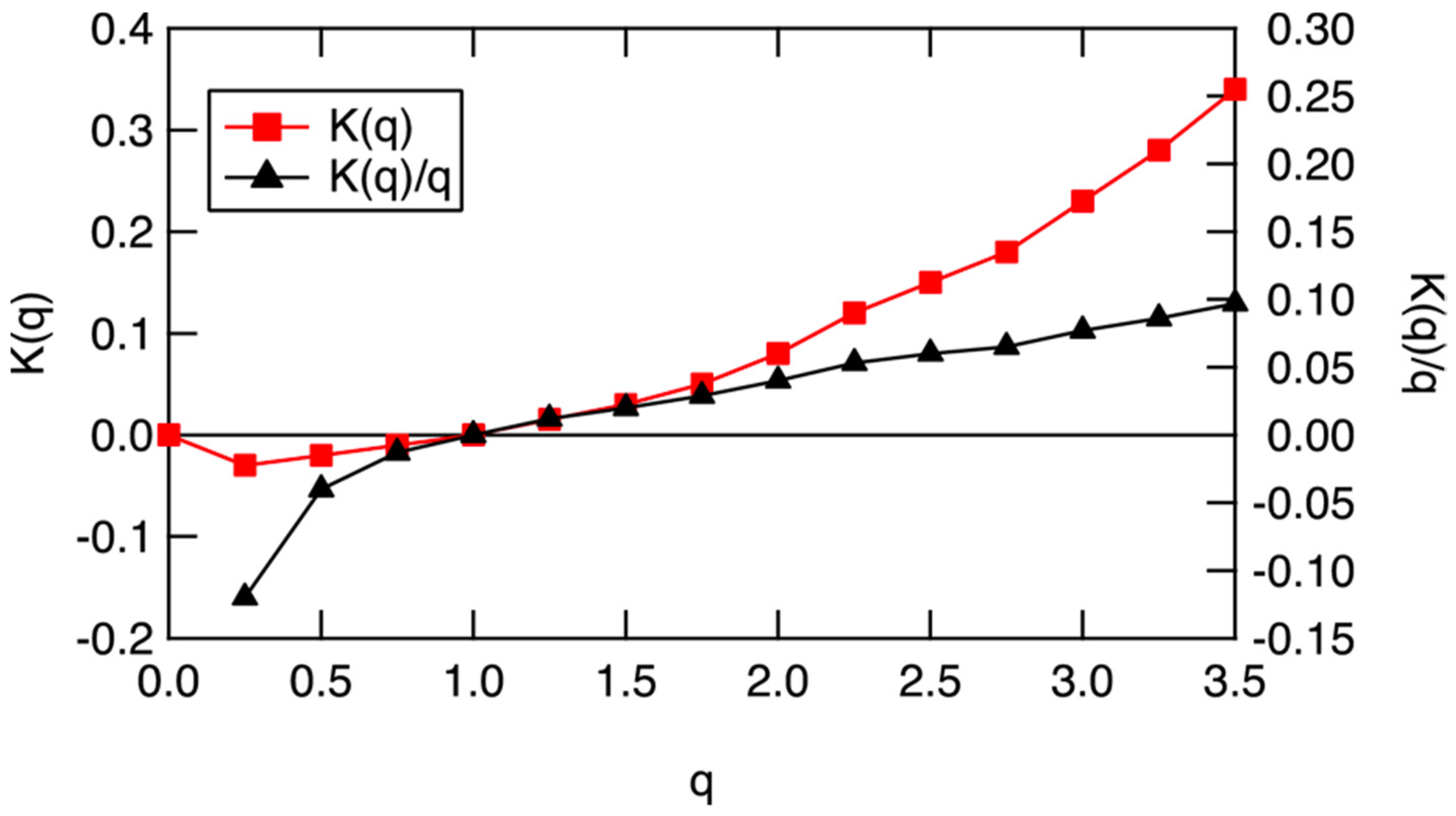
Figure 12. The scaling equivalent partition function K(q), left ordinate, and scaling equivalent Gibbs free energy, −K(q)/q, right ordinate, for the data in Figure 17. q = 1 is an indication of an approximate steady state, when both K(q) and K(q)/q are near zero. Heating will drive the air to higher values along the black curve, whereas cooling will drive it to lower values.
Figure 13. Probability distributions for molecules of velocity v evaluated according to the formulae given for most probable, average and root mean square values. Subtraction of the integral under the equilibrium black curve from that under the hypothetical non-equilibrium red curve should give the Gibbs free energy driving the circulation, and temperature via Equation (10).
This entry is adapted from the peer-reviewed paper 10.3390/meteorology1010003