Note：All the information in this draft can be edited by authors. And the entry will be online only after authors edit and submit it.

1.Introduction

These models typically focus on the joint evolution of a set of key biophysical variables using systems of coupled differential equations (although discrete time step models can also be used, as will be discussed below). These equations can be built from knowledge concerning the biophysical mechanisms underlying different forms of brain activity, or as phenomenological models chosen by the kind of dynamics they produce. Then, local dynamics are combined by in vivo estimates of anatomical connectivity networks. In particular, fMRI, EEG, and MEG signals can be used to define the statistical observables, diffusion tensor imaging (DTI) can provide information about the structural connectivity between brain regions by means of whole-brain tractography, and positron emission tomography (PET) imaging can inform on metabolism and produce receptor density maps for a given neuromodulator.

Most whole-brain models are structured around three basic elements:

• Brain parcellation: A brain parcellation determines the number of regions and the spatial resolution at which the brain dynamics take place. The parcellation may include cortical, sub-cortical, and cerebellar regions. Examples of well-known parcellations are the Hagmann parcellation [105], and the automated anatomical labeling (AAL) atlas [106].
• Anatomical connectivity matrix: This matrix defines the network of connections between brain regions. Most studies are based on the human connectome, obtained by estimating the number of white-matter fibers connecting brain areas from DTI data combined with probabilistic tractography [28]. For control purposes, randomized versions of the connectome (null hypothesis networks) may also be employed.
• Local dynamics: The activity of each brain region is typically determined by the chosen local dynamics plus interaction terms with other regions. A variety of approaches have been proposed to model whole-brain dynamics, including cellular automata [107,108], the Ising spin model [109,110,111], autoregressive models [112], stochastic linear models [113], non-linear oscillators [114,115], neural field theory [116,117], neural mass models [118,119], and dynamic mean-field models [120,121,122].

The first two items are guided by available experimental data. In contrast, the choice of local dynamics is usually driven by the phenomena under study and the epistemological context at which the modeling effort takes place. The workflow describing the construction of whole-brain models is illustrated in Figure 1. Because of this hybrid nature, whole-brain models constructed following this process are sometimes called semi-empirical models. Whole-brain models can be constructed from in-house code, or more easily from platforms, such as The Virtual Brain (https://www.thevirtualbrain.org/tvb/zwei) [30].

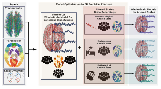
Figure 1. Workflow describing the construction of whole-brain models. First, model inputs are determined based on anatomical connectivity, a brain parcellation (representing a certain coarse graining), and the local dynamics (left). Each region defined by the parcellation is endowed with a specific connectivity profile and local dynamics. Then, the model can be optimized to generate data as similar as possible to the brain activity observed during conscious wakefulness. Generally, this similarity is determined by certain statistical properties of the empirical brain signals, which constitute the target observable. The same or another observable is obtained from subjects during altered states of consciousness and used again as the target of an optimization algorithm to infer model parameters. Following a given working hypothesis, the model for wakeful consciousness can be perturbed in such a way that optimizes the similarity between the target observable for the altered state of consciousness and the data generated by the model. In this way, a whole-brain model for an altered state of consciousness can be used to test working hypotheses about its mechanistic underpinnings.

2. Examples

2.1. Dynamic Mean-Field (DMF) Model

In this approach, the neuronal activity in a given brain region is represented by a set of differential equations describing the interaction between inhibitory and excitatory pools of neurons [125]. The DMF presents three variables for each population: the synaptic current, the firing rate, and the synaptic gating, where the excitatory coupling is mediated by NMDA receptors and the inhibitory by gamma-aminobutyric acid (GABA)-A receptors. The interregional coupling is considered excitatory-to-excitatory only, and a feedback inhibition control in the excitatory current equation is included [120]. The output variable of the model is the firing rate of the excitatory population that is then included in a nonlinear hemodynamical model [126] to simulate the regional BOLD signals.

The key idea behind the mean-field approximation is to reduce the high-dimensional randomly interacting elements to a system of elements treated as independent. Then, an average external field effectively replaces the interaction with all other elements. Thus, this approach represents the average activity of an homogeneous population of neurons by the activity of a single unit of this class, reducing in this way the dimensionality of the system. In spite of these approximations, the dynamic mean field model incorporates a detailed biophysical description of the local dynamics, which increases the interpretability of the model parameters.

2.2. Stuart-Landau Non-Linear Oscillator Model

This approach builds on the idea that neural activity can exhibit—under suitable conditions—self-sustained oscillations at the population level [107,114,115,124,127]. In this model, the dynamical behavior is represented by a non-linear oscillator with the addition of Gaussian noise at the proximity of a Hopf bifurcation [128]. By changing a single model parameter (i.e., bifurcation parameter) across a critical value, the model gives rise to three qualitatively different asymptotic behaviors: harmonic oscillations, fixed point dynamics governed by noise, and intermittent complex oscillations when the bifurcation parameter is close to the bifurcation (i.e., at dynamical criticality). Correspondingly, the model is determined by two parameters: the bifurcation parameter of the Hopf bifurcation in the local dynamics, and the coupling strength factor that scales the anatomical connectivity matrix. In contrast to the DMF model, coupled Stuart-Landau non-linear oscillators constitute a phenomenological model, i.e., the model parameter does not map into any biophysically relevant variables. In this case, the model is attractive due to its conceptual simplicity, which is given by its capacity to produce three qualitatively different behaviors of interest by changing a single parameter. 

3. How to Fit Whole-Brain Models to Neuroimaging Data?

Whole-brain models are tuned to reproduce specific features of brain activity. The way in which this is ensured is via optimization of the free parameters in the local dynamics plus the coupling strength. Parameter values are usually selected so that the model matches a certain statistical observable computed from the experimental data.

Since adding more free parameters increases the computational cost of the optimization procedure, it becomes critical to choose parameters reflecting variables that are considered relevant, either from a general neurobiological perspective or in the specific context of the altered state under investigation. Depending on the latter, the parameters could be divided into groups that are allowed to change independently based on different criteria, including structural lesion maps, receptor densities, local gene expression profiles, and parcellations that reflect the neural substrate of certain cognitive functions, among others.

After choosing the parcellation, the equations governing the local dynamics and their interaction terms, the interregional coupling given by the structural connectivity matrix, and selecting a criterion to constrain the dimensionality of the parameter space. The last critical step is to define the observable which will be used to construct the target function for the optimization procedure. As mentioned above, one possibility is to optimize the model to reproduce the statistics of functional connectivity dynamics (FCD). Perhaps a more straightforward option is to optimize the “static” functional connectivity matrix computed over the duration of the complete experiment, an approach followed by Refs. [115,124], among others. Other observables related to the collective dynamics can be obtained from the synchrony and metastability, as defined in the context of the Kuramoto model [115,130]. In general, any meaningful computation summarizing the spatiotemporal structure of a neuroimaging dataset constitutes a valid observable, with the adequate choice depending on the scientific question and the altered state of consciousness under study.

Since different observables can be defined, reflecting both stationary and dynamic aspects of brain activity, a natural question arises: is a given whole-brain model capable of simultaneously reproducing multiple observables within reasonable accuracy? We consider this question to be very relevant, yet at the same time it has been comparatively understudied.

Finally, some natural candidates for observables to be fitted by whole-brain models are precisely the high-level signatures of consciousness put forward by theoretical predictions. The objective is to fit whole-brain models using these signatures as target functions and then assess the biological plausibility of the optimal model parameters, which allows for the testing of the consistency of these signatures from a bottom-up perspective. Alternatively, signatures of consciousness can be computed from the model—initially fitted to other observables—and compared to the empirical results. Again, this highlights the need to understand which kind of local dynamics allow the simultaneous reproduction of multiple observables derived from experimental data.

4. Whole-Brain Models Applied to the Study of Consciousness

The available evidence suggests that states of consciousness are not determined by activity in individual brain areas, but emerge as a global property of the brain, which in turn is shaped by its large-scale structural and functional organization [53,131,132]. According to this view, whole-brain models provide a fertile ground to explore how global signatures of different states of consciousness emerge from local dynamics. This promise is already being met, as shown by several recent articles [38,107,114,115,123,124,127,133].

Another interesting possibility is to assess the consequences of stimulation protocols that are impossible to apply in vivo. An example is the Perturbative Integration Latency Index (PILI) [127], which measures the latency of the return to baseline after a strong perturbation that generates dynamical changes detectable over long temporal scales (on the order of tens of seconds). This in silico perturbative approach allows to systematically investigate how the response of brain activity upon external perturbations is indicative of the state of consciousness, providing new mechanistic insights into the capacity of the human brain to integrate and segregate information over different time scales.

This entry is adapted from the peer-reviewed paper 10.3390/brainsci10090626