Bioacoustic Detection of Wolves

Bioacoustic Detection of Wolves: History

Please note this is an old version of this entry, which may differ significantly from the current revision.

Subjects: Others

Contributor:

Wolves (Canis lupus) are generally monitored by visual observations, camera traps, and DNA traces. However, several studies use acoustic devices to monitor wolves.

bioacoustics
Canis lupus
discriminant analysis
habitats directive

1. Introduction

In 2012, a wolf (Canis lupus lupus) was found dead in northern Jutland, Denmark, which was the first observation of wolves in Denmark since 1813 [1]. The wolves in Denmark are dispersers from Germany and their descendants, and are part of a connected Central European wolf population. In Europe (excluding Russia), there are more than 17,000 wolves [2]. In the European Union (EU), the wolf population is estimated to exceed 13,000 individuals [2] and the European populations are generally increasing in size due to recent protection. However, in most Western European countries the populations are still relatively small with less than 1000 wolves [1,2]. In Scandinavia, the population is approximately 480 wolves [3], and there are at least a further 780 individuals found in Germany and western Poland [2]. Wolves dispersing from the Central European population have reached Belgium, the Netherlands, and Denmark [1,2]. The number of wolves present in Denmark was estimated as a litter of 4 pups and 11 adult individuals in the period 1 April to 30 June 2021; in total, it was estimated that there were eight immigrant adults and seven Danish born individuals [4]. However, monitoring the population and dispersal of individuals has proved to be challenging as wolves are both wide-ranging [5,6] and notoriously fearful of humans [7].

As in the rest of Europe, Denmark is obligated to monitor wolves according to the EU Habitats Directive (92/43/EEC) [8]. In Scandinavia and Germany, databases containing validated wolf observations, reported by citizens and by volunteers, and DNA samples obtained from scats and the carcasses of killed domestic animals have been established to track the population status of wolves [9,10,11]. A genetic reference database for wolves in Central Europe has been established to analyze the origin and movements of wolves across Europe [12].

Currently there is both active and passive monitoring of wolves in Denmark [1,13]. Active monitoring consists of registering tracks and DNA profiles, and the use of camera traps [14,15]. Passive monitoring is the registration of public observations, including organized volunteers as part of citizen science projects [14,15]. Camera traps are an essential tool but are limited by their small field of view compared to wolves’ extensive physical range, and their effective deployment requires prior knowledge of wolf presence in an area.

Acoustic monitoring is a passive monitoring tool that has been used in the last decades for studies of diverse taxa, including insects [16], bats [17,18], birds [19], whales [20,21], and large terrestrial mammals such as ungulates [22,23] and elephants [24], and with acoustic devices; it is similarly possible to detect elusive but vocal species such as wolves [25]. Recognizing individual wolves on their howls can give insight into their movements and territory size. Several studies have shown that acoustic monitoring of wolves can be a useful and relevant tool since it is cost-effective and non-invasive [26,27,28,29,30] and can help recognize wolves from a distance and determine the number of wolves present [25,28,30,31,32].

Acoustic monitoring of wolves is based in detection of their howls [26,33,34]. Wolves use howls for different purposes: (1) to defend their territory [26,33,35], (2) to contact members of the pack [26,35], and (3) to socialize [33,35]. They may howl solo or in chorus from packs [26,36]. Wolves usually howl around twilight and in the middle of the night [35] and their emissions are most intense during the months of July through October, when the presence of pups increases the pack’s howling [33]. This is likely to make other predators aware that the pups are protected by adults [33].

The fundamental frequency (f0) is the lowest frequency band of the tonal call as wolf howl. For wolves, the f0 typically has values between 150 and 780 Hz [37] and has been used to identify individual wolves with high accuracy within subspecies of wolves such as Eastern wolves (Canis lupus lycaon) [27,38], Indian wolves (C. l. pallipes) [39], and Iberian wolves (C. l. signatus) [36]. Root-Gutteridge et al. [40] were able to identify individuals in captive Eastern wolves with 100% accuracy using both f0 and amplitude (the highest variation of a wave in air pressure, perceived as volume). The use of amplitude for encoding individual identity for wolves in situ requires additional studies to determine the rate of sound suppression over distance, in different weather conditions, and through different habitats such as open land or forest [27]. Furthermore, wolves have been shown to have different vocal signatures depending on the subspecies [32,41] and are group specific [42].

Monitoring based on camera traps requires individuals in near field of view, which are most efficient at 10 m [43], whereas acoustic recorders cover larger distances with a with a radius of 3 km [28]. However, development of the methodology for analyzing the acoustic data is essential for wider scale use. Because of the small population in Denmark, captive wolves located in zoos are of importance to train the algorithm to recognize wolf howls. We know numbers present and can recognize individuals in zoos. Additionally, subspecies are known to show variations in their howls [41]; thus, recognition should be trained on the relevant subspecies.

2. Identification of Subspecies

All the 170 howls from the seven wolves were used in the analysis for subspecies. The discriminant analysis using nine acoustic variables (Maxf0, Posmaxf0, Sd, Slope, Cofm, IQR, Startf0, Endf0, and Duration) gave an overall 78% of correctly classified subspecies (Figure 1). For Northwestern wolves the classification was 64%, for Arctic wolves, the classification was 82%, and finally for Eurasian wolves it was 77%. Pairwise post-hoc Hotelling test analysis showed significant difference in howls between Arctic and Eurasian wolves (DF = 9, F = 23.77, p < 0.001), Arctic and Northwestern wolves (DF = 9, F = 2.9, p < 0.01), and Eurasian and Northwestern wolves (DF = 9, F = 10, p < 0.001) all p-values were significant after sequential Bonferroni correction (Table 1). The randomized subsets gave overall correct classifications between 70% and 90% where most were between 82% and 88%. Pairwise post-hoc Hotelling test showed significant differences between most randomized subsets. After sequential Bonferroni 72% was not significant.

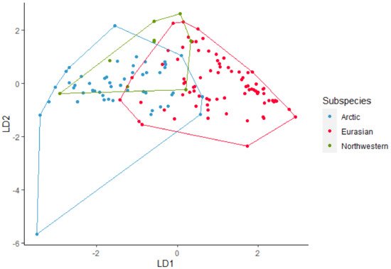
Figure 1. Linear discriminant (LD) analysis plot for identification of the subspecies Arctic, Eurasian, and Northwestern wolves with a 78% correct classification.

Table 1. Pairwise post-hoc Hotelling test for Subspecies with F-values, p-values, and number of degrees of freedom (DF). Symbol ^# indicates significant p-values after sequential Bonferroni.

	F	p	DF
Arctic-Eurasian	23.77	<0.001 ^#	9
Arctic-Northwestern	2.9	<0.01 ^#	9
Eurasian-Northwestern	10	<0.001 ^#	9

3. Individual Identification of Arctic Wolves

Sixty-two howls from four wolves were used in the analysis of howls from Arctic wolves. The discriminant analysis using eight variables (Minf0, Maxf0, Posmaxf0, Sd, Cofm, Startf0, Endf0, and Duration) gave an overall 95% correct classification of howls from the four wolves (Figure 2). Classification of each wolf showed that RW1, RW2 and WCTM all have 100% correct classification and WCTF has a 91% correct classification. The pairwise post-hoc Hotelling test showed significant difference in howls between RW1 and RW2 (DF = 8, F = 33.2, p < 0.001), between howls from RW1 and WCTM (DF = 8, F = 37.52, p < 0.001), between RW2 and WCTM (DF = 8, F = 9.68, p < 0.01), between RW1 and WCTF (DF = 8, F = 93,87, p < 0.001), between RW2 and WCTF (DF = 8, F = 41.74, p < 0.001) and lastly between WCTM and WCTF (DF = 8, F = 8.2, p < 0.01). All pairwise post-hoc Hotelling tests showed significant differences after sequential Bonferroni were applied (Table 2). After randomizing the data, the correct classification ranged between 89% and 100%, where most lay between 94% and 97%. The pairwise post-hoc Hotelling tests for the randomized subsets showed significant differences with all subsets of RW1 after sequential Bonferroni correction. The pairwise post-hoc Hotelling test showed significant differences between RW2 and WCTM. However, after sequential Bonferroni correction 70% was not significant. The pairwise post-hoc pairwise post-hoc Hotelling tests for randomized RW2 and WCTF showed significant difference in howls for all subsets. After sequential Bonferroni correction 80% was significant. The pairwise post-hoc Hotelling for randomized WCTM and WCTF showed significant differences for most subsets. After sequential Bonferroni correction 70% was not significant.

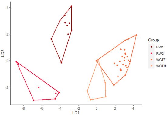
Figure 2. Linear discriminant (LD) analysis plot for individual identification of howls from Arctic wolves with a 95% correct classification.

Table 2. Pairwise post-hoc Hotelling test for Arctic wolves with F-values and p-values. Symbol ^# indicates significant p-values after sequential Bonferroni test.

	F	p	DF
RW1-RW2	33.2	<0.001 ^#	8
RW1-WCTM	37.52	<0.001 ^#	8
RW1-WTCF	93.87	<0.001 ^#	8
RW2-WCTM	9.68	<0.01 ^#	8
RW2-WCTF	41.74	<0.001 ^#	8
WCTM-WCTF	8.2	<0.01 ^#	8

4. Individual Identification of Eurasian Wolves

Ninety-seven howls from nine Eurasian wolves were used in this analysis. Using eight variables (Minf0, Maxf0, Posmaxf0, Sd, Cofm, Startf0, Endf0, and Duration), the discriminant analysis achieved 89% accurate classification (Figure 3). SK1, and ULF achieved 100% correct classification. BLS0028 achieved a correct classification of 94%, BLS011 had an 85% correct classification. BLS026 achieved 83% correct classification and BLS010 achieved an 82% correct classification. The pairwise post-hoc Hotelling test showed significant differences between howls from all except BLS011 and BLS026 (Table 3). After sequential Bonferroni correction BLS026 and SK1 and BLS011 and SK1 were not significant. After randomizing the data, the correct classification ranged between 89% and 97%, where most were between 92% and 97%. The pairwise post-hoc Hotelling test revealed 57% significant differences and 20% was significant after sequential Bonferroni correction was applied.

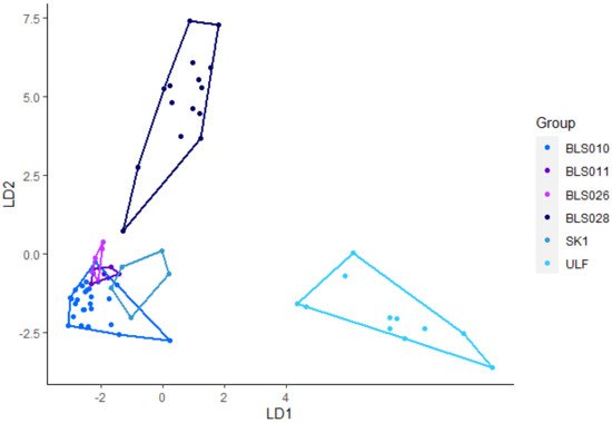
Figure 3. Linear discriminant (LD) analysis plot for individual identification of howls from Eurasian wolves with a 92% correct classification.

Table 3. Pairwise post-hoc Hotelling test for Arctic wolves with F-values, p-values and number of degrees of freedom (DF). Symbol ^# indicates significant p-values after sequential Bonferroni. n.s. indicates not significant p-values.

	F	p	DF
BLS010-BLS011	8.05	<0.001 ^#	7
BLS010-BLS026	13.91	<0.001 ^#	7
BLS010-BLS028	62.04	<0.001 ^#	7
BLS010-SK1	58.31	<0.001 ^#	7
BLS010-ULF	169.04	<0.001 ^#	7
BLS011-BLS026	1.56	n.s.	7
BLS011-BLS028	9.21	<0.001 ^#	7
BLS011-SK1	23.07	<0.01 ^#	7
BLS011-ULF	32.85	<0.001 ^#	7
BLS026-BLS028	10.2	<0.001 ^#	7
BLS026-SK1	9.61	<0.05	7
BLS026-ULF	34.13	<0.001 ^#	7
BLS028-SK1	17.44	<0.001 ^#	7
BLS028-ULF	37.4	<0.001 ^#	7
SK1-ULF	13.16	<0.001 ^#	7

This entry is adapted from the peer-reviewed paper 10.3390/ani12050631

© Text is available under the terms and conditions of the Creative Commons Attribution (CC BY) license; additional terms may apply. By using this site, you agree to the Terms and Conditions and Privacy Policy.