Benchmark calculations of high-precision numerical scheme for nonlinear hyperbolic evolution equations are demonstrated. The scheme is based on the Fourier spectral method for the spatial discretization and the implicit Runge-Kutta method for time discretization.
- benchmark calculations
- high-precision numerical scheme
- hyperbolic evolution equation
- Klein-Gordon equation
- Sine-Gordon equation
1. Nonlinear hyperbolic evolution equations
The dynamics of nonlinear hyperbolic equations are fascinating enough to be applicable to wave propagation in any scales from elementary particles to waves in cosmic scale. Even fundamental properties have not been fully understood for nonlinear hyperbolic problems, and it is difficult to elucidate these properties only by pure mathematical analysis. So that to understand fundamental properties of nonlinear waves, it is useful to employ numerical calculations. Note that, while in terms of treating various nonlinear problems (e.g., various type of boundary, discontinuity such as shock propagation) it is practical to specialize numerical schemes individually, a basic and general framework for precisely calculating nonlinear hyperbolic evolution equations had not been well established until Takei-Iwata [1]. Here some benchmark calculations of high-precision numerical scheme for calculating nonlinear hyperbolic evolution equations are demonstrated. Much attention is paid to “universal applicability” and “reliability”. Among others, demonstration movies are presented in this article for the first time.
For a concrete problem, we consider one-dimensional nonlinear Klein-Gordon equations (for a textbook, see [2]). The initial and boundary values problem of one-dimensional Klein-Gordon equations is written by

for (x, t) ∈ [0, L] × [0, T], where α, β and T are real numbers, and f (x) and g(x) are initial functions. The periodic boundary condition is imposed. Inhomogeneous term F(u) is either linear or nonlinear function of u (e.g., the polynomials or trigonometric functions of u). For constructing the numerical scheme, the equations are written by a system of first-order evolution equations:

2. Background: challenges in numerical computation
Various numerical schemes have been investigated to reproduce the solutions of nonlinear partial differential equations accurately and efficiently. For nonlinear hyperbolic equations, numerical schemes well reproducing the conservation laws is required to be highly accurate, since the smoothing effect particularly associated with parabolic equations cannot be expected. Here, when typical numerical schemes such as the difference method are applied, we face various problems in the discretization of spatial and time variables as shown below.
2.1. Spatial discretization
For the spatial discretization, a conventional finite difference method can be used to discretize the spatial variables in calculating Klein-Gordon equations, but it requires a very small spatial unit Δx to ensure the sufficient accuracy. Furthermore, the numerical dispersion inevitably appears in typical finite difference methods in which numerical solutions are known to be difficult to satisfy the conservation laws with certain sufficient accuracy.
2.2. Time discretization
For the time discretization, explicit methods have been usually employed in calculating Klein-Gordon equations, but it requires additional treatments to obtain sufficiently accurate solutions. While linear and nonlinear solvers based on explicit methods are relatively simple with low computation cost, it is also known that there is a restriction called the Courant-Friedrichs-Lewy Condition (CFL condition, for short) on the time unit Δt in order to obtain numerical results stably. Therefore, a numerical scheme combining explicit and implicit methods has been studied: e.g., a method for weakening the restriction on Δt with keeping the stability of calculations [3-5].
2.3. High-precision numerical scheme
For a high-precision numerical scheme, here we present spectral method for spatial discretization and Runge-Kutta method for time discretization [1]. By the spectral method, the solution in the wavenumber space is efficient to avoid the numerical dispersion, and to satisfy conservation laws to certain satisfactory degrees. By the two-stage and third-order Runge-Kutta method as unconditionally-stable fully implicit method, the numerical solution with high accuracy can be necessarily obtained stably. The calculation cost of numerical scheme is small enough to be at the order of O(N log2 N). The precision of the scheme can be found in Fig. 1.
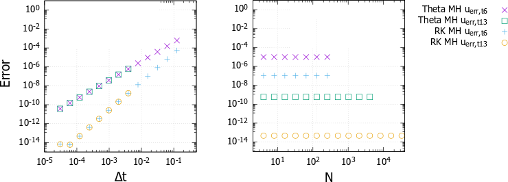
Figure 1. Δt (left panel) and Δx (right panel) dependence of error, where Δx-1 is parametrized by N. The proposed scheme corresponds to RK MH uerr, t13 (for details of notation, see [1]).
3. Details of numerical scheme
3.1. Fourier spectrum method
The spectral method [8-13] is employed for discretizing the spatial variable. Let the solution of Eq. (2) be expanded by the Fourier series
Then substitute them into the first equation of (2). After multiplying cos(2πkx/L) and sin(2πkx/L) respectively, they are integrated over Ω = [0, L] with respect to x. Similarly, substitute Eq. (3) into the second equation of (2). After multiplying cos(2πkx/L) and sin(2πkx/L) respectively, they are integrated over Ω = [0, L] with respect to x. The unknowns are formulated as
The equations are written by
In each time step, the solution to the original Eq. (2) is obtained by solving Eqs. (4) and (5) in which a0, c0 and al , bl , cl , dl (l = 1, ・ ・ ・ , N) are calculated.
3.2. Implicit Runge-Kutta method
The implicit Runge-Kutta method [14] of two-stage and third-order is employed for discretizing the time variable. Let u(t) be the solution of the initial value problem of the abstract evolution equation

in a Hilbert space. The time interval (α, β) is divided into equally-discretized M segments being incremented by Δt = (β - α)/M. Let the discrete time sequence {tm} be represented by

and the approximated value of unknown function u(tm) be denoted by Um. In this situation, the following method for obtaining the approximate value Um+1 is called the Runge-Kutta method

Here, the natural number s is called the number of steps, and ai j, bi, ci are the parameters that define the formula. It is called the implicit Runge-Kutta method when ai j≠0 (j > i) exists. The conditions

are imposed on the parameters ai j, ci.
4. Demonstration of high-precision numerical scheme
4.1. Example: linear case (video)
Let us take the initial and boundary value problem (2) with F(u) = u, α = -1, β = 1, Ω = [0, L].
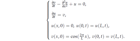
The initial function is shown in Figure 2, and the calculated movie is shown in Video 1 and Video 2.
Figure 2. Initial function u and v.
4.2. Example: nonlinear case (video)
Let us take the initial and boundary value problem (2) with F(u) = sin u, α = -1, β = 1, Ω = [0, L], L= 6.7430014192503. The nonlinear wave equation in this case is known as the Sine Gordon equation.
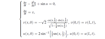
The initial function is shown in Figure 3, and the calculated movie is shown in Video 3 and Video 4.
Figure 3. Initial function u and v.
4.3. Example: other cases with high complexity
In addition, the calculation results of more complicated solutions such as the breather solution for nonlinear hyperbolic equations can be found in Refs. [6-7].
References
- Y. Takei, and Y. Iwata, “Numerical scheme based on the implicit Runge-Kutta method and spectral method for calculating nonlinear hyperbolic evolution equations”, Axioms 2022, 11 (1), 28.
- J. D. Bjorken, and S. D. Drell, “Relativistic quantum fields”, MacGraw-Hill, 1965.
- I. Cordero-Carrion and P. Cerda-Duran, “Partially implicit Runge-Kutta methods for wave-like equations", F. Casas, V. Martinez (eds.), Advances in Differential Equations and Applications, SEMA SIMAI Springer Series 4, 2012.
- H. Wang, Q. Zhang and C.-W. Shu, “Third order implicit-explicit Runge-Kutta local discontinuous Galerkin methods with suitable boundary treatment for convection diffusion problems with Dirichlet boundary conditions", Journal of Computational and Applied Mathematics, 342, pp.164-179, 2018.
- W. Zhao and J. Huang, “Boundary treatment of implicit-explicit Runge-Kutta method for hyperbolic systems with source terms", Journal of Computational Physics, 423 (15), 2020.
- Y. Takei, Y. Iwata, "Space-time breather solution for nonlinear Klein-Gordon equations", J. Phys.: Conf. Ser. 1730, 2021.
- Y. Takei, Y. Iwata, "Stationary analysis for coupled nonlinear Klein-Gordon equations", submitted, 2021; arXiv:2109.11038.
- J. P. Boyd, “Chebyshev and Fourier Spectral Methods Second Edition (Revised)", Dover, 2001.
- B. Fornberg, "A Practical Guide to Pseudospectral Methods", Cambridge University Press, 1995.
- D. Gottlieb and S. A. Orszag, “Numerical Analysis of Spectral Methods: Theory and Applications", SIAM-CBMS, 1997.
- C. Canuto, M. Y. Hussaini, A. Quarteroni, and T. A. Zang, “Spectral Methods in Fluid Dynamics", Springer-Verlag, 1986.
- Y. Iwata, Y. Takei, “Numerical scheme based on the spectral method for calculating nonlinear hyperbolic evolution equations", Research Reports of Kanagawa Institute of Technology B(44), pp.1-8, 2020; in Japanese, doi: 10.34411/00032023.
- Y. Iwata, Y. Takei, “Numerical scheme based on the spectral method for calculating nonlinear hyperbolic evolution equations", ICCMS ’20: Proceedings of the 12th International Conference on Computer Modeling and Simulation, pp.25-30, ACM Digital Library (ISBN: 978-1-4503-7703-4) 2020.
- J. C. Butcher, “The Numerical Analysis of Ordinary Differential Equations: Runge-Kutta and General Linear Methods", John Wiley and Sons, 1987.