1.Publishing time

Figure 1 shows the number of publications from 2011 to November 2021, for 71 models. Although this is not all the literature, the search results are sorted by relevance, and the data in the figure is still representative and reliable. The figure shows that from 2011 to 2015, the research progress of using intelligent models to predict remaining strength and remaining life was relatively stable. Although there was a sharp decline in 2016-2018, the overall trend was stable. After 2019, related research showed a spurt of growth. It can be inferred that the prediction of remaining strength and remaining life is still a research hot spot.

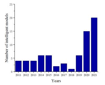
Figure 1. The number of related intelligent models from 2011 to November 2021.

2.Result analysis of traditional evaluation methods

Due to the differences of various evaluation methods in many aspects ^[1], the calculation results also be affected. 64 groups of data were collected, including 40 groups of low-strength steel grade corrosion pipes (X42, X46-1, X46-2, X46-3, X46-4, X52-1, X52-2, X56) and 24 groups of medium and high-strength steel grade corrosion pipes (X60, X65, X80), including defect size parameters, pipe size parameters, material parameters and burst test pressure. The result analysis of various evaluation methods is shown in figures (Figure 2, Figure 3, Figure 4, Figure 5). As the figures shown, ASME B31G has large errors in evaluating whether it is a medium-to-high strength pipeline or a low-strength pipeline. The Modified B31G has improved significantly. When evaluate low-strength steel pipes, DNV-RP-F101 allowable stress method and PCORRC have similar errors. However, when evaluating high-strength steel-grade pipelines, the accuracy of DNV-RP-F101 allowable stress method is much higher than that of PCORRC.

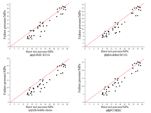
Figure 2. Comparison of burst pressure and predicted failure pressure of low-strength pipelines calculated by different methods. (a) ASME B31G; (b) Modified B31G; (c) Allowable stress; (d) PCORRC.

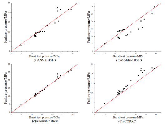
Figure 3. Comparison of burst pressure and predicted failure pressure of medium and high strength pipelines calculated by different methods. (a) ASME B31G; (b) Modified B31G; (c) Allowable stress; (d) PCORRC.

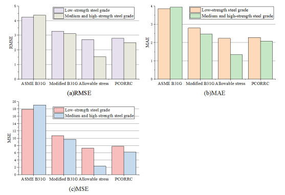
Figure 4. Errors in calculating failure pressure of corroded pipelines of low, medium and high strength steel grades by different methods. (a) RMSE; (b) MAE; (c) MSE.

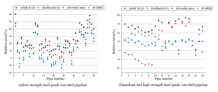
Figure 5. Different methods to calculate relative error of failure pressure of (a) low-strength steel grade corroded pipeline; (b) high-strength steel grade corroded pipelines.

3.Prediction accuracy

Error indicator can be used to evaluate the performance of prediction model [^[2],^[3],^[4],^[5],^[6]]. By counting the indicators used in the discussed models, this paper summarizes 18 indicators used to evaluate the prediction accuracy. Figure 6 indicates that the most frequently used error indicators are MSE, R², MAPE, RMSE and MAE. Among these indicators, MSE, RMSE, and MAE have no benchmark because the data dimension because the datasets dimensions are different. MAPE and R² can be compared in different usage scenarios because they reflect relative errors. The closer R² is to 1, the higher the prediction accuracy. The smaller the MAPE, the higher the prediction accuracy. MAPE and R² in residual strength and residual life prediction models are counted in the Table 1. Among the 71 models, the range of MAPE is between 0.0123 and 0.1499, the range of R² is between 0.619 and 0.999. Lewis once gave a reference, when the MAPE is less than 0.1, the model performance is excellent; when the MAPE is greater than 0.1 and less than 0.2, the model performance is good; when the MAPE is greater than 0.2 and less than 0.5, the model performance is reasonable; when the MAPE is greater than 0.5, the model is not suitable.

Table 1. MAPE and R2 statistics of residual strength and residual life forecasting results.

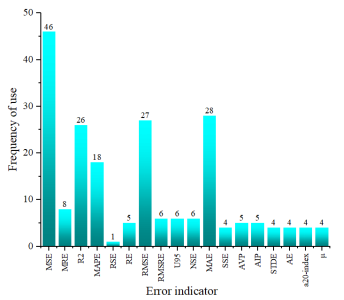
Figure 6. The frequency of using various error indicators in 71 models.

4.Data size and data division

Data size is one of the main factors affecting forecasting performance. Too much data will lead to too much calculation, while too little data may lead to the insufficient model accuracy. Table 2 provides statistical information on the data size of 71 smart models, which can provide a basis for selecting data sizes in subsequent studies. The original data is usually divided into three data sets in machine learning, including training set, validation set, and test set. The training set is used to train the model; the validation set data is used to adjust the parameters of the training model; the test set data is used to measure the performance of the training model. However, only 2 of the 71 models divide the original data into three data sets, and the remaining 69 models only divide it into the training and test sets (Figure 7). The proportion of test set is in the range of 0.015-0.4.

Table 2. The data size of prediction models.

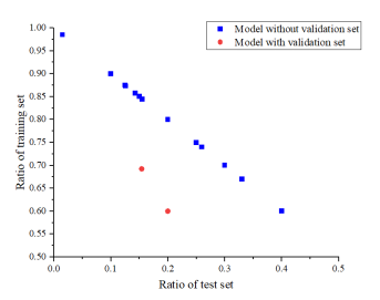
Figure 7. Division proportion of raw data.

5.Input variable and output value

In the intelligent model, how to determine the input variables is a very critical issue [^[7],^[8]]. Therefore, in the remaining strength and remaining life prediction model, it is necessary to consider which factors are used as input variables fully. According to the input variables, it can be divided into two categories. One is to simply use a certain historical data as an input variable to predict the future trend of the variable, such as using the historical wall thickness of the pipeline to predict the remaining wall thickness and using the historical corrosion rate to predict the future corrosion rate. The other is the prediction that considers multiple factors, such as predicting the burst pressure of the pipeline through pipeline size parameters, defect parameters, environmental parameters, and material parameters (Table 3). The former is simple to calculate and convenient to obtain data, but the prediction accuracy is not necessarily high, because this type of prediction assumes that external factors are stable. The latter is difficult to obtain data and needs to consider the nonlinear relationship of multiple variables, but the prediction results are often more comprehensive and accurate. According to the statics of the models compiled in this paper,10 of the 71 models are simple time-series predictions, and the rest are forecasting considering multiple factors.

Table 3. The input variables of prediction models.

The prediction targets of these models can be roughly divided into the following four categories: burst pressure, remaining thickness, corrosion rate and others. Among them, burst pressure accounts for 36%, remaining thickness accounts for 18.7%, corrosion rate accounts for 21.3%, corrosion defect depth accounts for 6.7% and the others accounts for 17.3%. The proportion of each item is shown in Figure 8. It can be seen from Figure 8 that the model with burst pressure as the output value is still the most, the rest are similar.

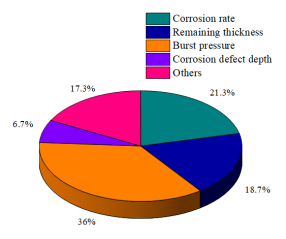
Figure 8. Output value of 71 models.

This entry is adapted from the peer-reviewed paper 10.3390/en15030726

References

- A Syrotyuk; Karpenko Physico-Mechanical Institute of the National Academy of Sciences of Ukraine; O Vytyaz; J Ziaja; AGH University of Science and Technology; Damage to flexible pipes of coiled tubing equipment due to corrosion and fatigue: methods and approaches for evaluation. Mining of Mineral Deposits 2017, 11, 96-103, 10.15407/mining11.04.096.
- Hongfang Lu; Tom Iseley; John Matthews; Wei Liao; MohammadAmin Azimi; An ensemble model based on relevance vector machine and multi-objective salp swarm algorithm for predicting burst pressure of corroded pipelines. Journal of Petroleum Science and Engineering 2021, 203, 108585, 10.1016/j.petrol.2021.108585.
- Zhao-Dong Xu; Chen Zhu; Ling-Wei Shao; Damage Identification of Pipeline Based on Ultrasonic Guided Wave and Wavelet Denoising. Journal of Pipeline Systems Engineering and Practice 2021, 12, 04021051, 10.1061/(asce)ps.1949-1204.0000600.
- Hongfang Lu; Tom Iseley; John Matthews; Wei Liao; Hybrid machine learning for pullback force forecasting during horizontal directional drilling. Automation in Construction 2021, 129, 103810, 10.1016/j.autcon.2021.103810.
- Zhao-Dong Xu; Yang Yang; An-Nan Miao; Dynamic Analysis and Parameter Optimization of Pipelines with Multidimensional Vibration Isolation and Mitigation Device. Journal of Pipeline Systems Engineering and Practice 2021, 12, 04020058, 10.1061/(asce)ps.1949-1204.0000504.
- Hongfang Lu; John C. Matthews; MohammadAmin Azimi; Tom Iseley; Near Real-Time HDD Pullback Force Prediction Model Based on Improved Radial Basis Function Neural Networks. Journal of Pipeline Systems Engineering and Practice 2020, 11, 04020042, 10.1061/(asce)ps.1949-1204.0000490.
- Shanbi Peng; Ruolei Chen; Bin Yu; Min Xiang; Xiugao Lin; Enbin Liu; Daily natural gas load forecasting based on the combination of long short term memory, local mean decomposition, and wavelet threshold denoising algorithm. Journal of Natural Gas Science and Engineering 2021, 95, 104175, 10.1016/j.jngse.2021.104175.
- Hongfang Lu; Saleh Behbahani; Xin Ma; Tom Iseley; A multi-objective optimizer-based model for predicting composite material properties. Construction and Building Materials 2021, 284, 122746, 10.1016/j.conbuildmat.2021.122746.