Your browser does not fully support modern features. Please upgrade for a smoother experience.
Please note this is an old version of this entry, which may differ significantly from the current revision.
Subjects:
Orthopedics
A convolutional neural network (CNN) is a deep learning algorithm architecture created based on a 1962 study investigating the visual process of feline brains, and it has been applied in a wide range of areas, from autonomous vehicles to medical diagnoses. Since 2017, many studies applying deep learning-based diagnostics in the field of orthopedics have demonstrated outstanding performance.
- artificial intelligence
- orthopedics
- neural network
- deep learning
1. Introduction
A convolutional neural network (CNN) is a deep learning algorithm architecture created based on a 1962 study investigating the visual process of feline brains, and it has been applied in a wide range of areas, from autonomous vehicles to medical diagnoses [1].
A traditional CNN consists of an input layer that transmits input information, a hidden layer that modifies information (filtering) received from the input layer and amplifies the features (pooling) and an output layer that finally synthesizes and outputs the information.
According to the universal approximation theorem, it has been confirmed that various linear classifications are possible even if the neural network has a shallow hidden layer, and some pioneering studies have shown that classification and detection are improved as the layers constituting the neural network become deeper (deep neural network) [2]. Since 2012, the performance of deep learning has rapidly increased in medical image analysis with the use of deep neural networks, and this has led to a decrease in the classification error rate from approximately 25% in 2011 to 3.6% in 2015.
The CNN model was developed using a pipeline in terms of classification and detection [3], and the improved CNN shows excellent judgment, essentially giving the computer a new visual organ. A CNN has thus been expected to be used for medical diagnoses. However, a CNN does not provide any information on the basis of the decision. Therefore, even if a CNN shows an excellent diagnostic ability, it can only be discussed within a limited scope in medicine, where the basis for a judgment is important [4].
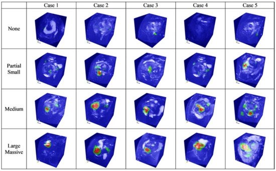
This has been pointed out as a technical limitation that reduces the effectiveness of a CNN in various fields other than medicine [5]. Researchers have dubbed this limitation “black box issues” and worked to develop “explainable artificial intelligence (XAI)” to look inside the problem [6]. The term “explainable” can be expressed as “understandability”, “comprehensibility” or “interpretability” and has the same meaning. XAI should not degrade the classification or prediction performance of the model in any way and should improve the explainability. Various strategies and suitable CNN architectures have been proposed to implement an appropriate XAI [7]. Unfortunately, the black box nature of deep learning has not been completely resolved, but there are some notable achievements [8]. As one of these achievements, in 2016, Zhou et al. introduced a method explaining how a CNN makes a decision through class activation mapping [9], and this method is widely used in the field of medical artificial intelligence (Figure 1) [10].

Figure 1. Image highlighting the location and size of a rotator cuff tear through a class activation map (CAM). Figure obtained from a study performed by Chung et al. [10].
In a similar context, there are attempts to improve the explainability by improving the existing CNN architecture [11]. Kim et al. modified U-Net, a CNN architecture that has strength in image segmentation, to appropriately increase the explainability. They presented an interpretable version of U-Net (SAU-Net) using an attention module for the decoder part [12].
Hence, studies introducing CNN models for diagnosing and classifying diseases using deep learning have been published in various fields of medicine, including ophthalmology and dermatology [13,14].
2. Deep Learning for Fractures
Fractures are the most familiar ailments to orthopedists and the medical area in which deep learning methods were first applied. In 2018, Chung et al. published a CNN model for diagnosing and classifying proximal humerus fractures. Three specialists labeled 1891 anteroposterior shoulder radiographs as normal shoulders (n = 515) and 4 proximal humerus fracture types (greater tuberosity: 346; surgical neck: 514; 3-part: 269; and 4-part: 247) [15]. After labeling, a CNN model (ResNet-152) was trained with a training dataset created through augmentation of the labeled data. The CNN model recorded 96% accuracy for the normal shoulders and proximal humerus fractures, showing a higher accuracy than a general orthopedist (92.8% accuracy). This model showed a top-1 accuracy of 65–86% and an area under the curve (AUC) of 0.90–0.98 for classifying the fracture types. A recently published paper introduced a model with improved classification accuracy. In 2020, Demir et al. introduced a deep learning model to diagnose and classify humerus fractures using the exemplar pyramid method, a novel, stable feature extraction approach which showed a high classification accuracy of 99.12% [16].
Urakawa et al. trained the VGG-16 CNN model using hip plain radiographs (1773 intertrochanteric hip fracture images and 1573 normal hip images) and showed an accuracy of 95.5% [17]. Yamada et al. trained the CNN model (Xception architectural) based on 3123 hip plain and lateral radiography images, and the trained model classified fractures with 98% accuracy, which is better than orthopedists (92.2% accuracy) [18].
For the hip, as with the shoulder, there has been an attempt to classify fractures by training the CNN model. Lee et al. introduced a CNN model for training 786 anteroposterior pelvic plan radiographs using GoogLeNet-inception v3 [19]. The model classified a proximal femur fracture into type A (trochanteric region), type B (femur neck) and type C (femoral head) according to AO/OTA classification with an overall accuracy of 86.8%, showing a reasonable result. Lind et al. trained a ResNet-based CNN with anteroposterior and lateral knee radiographs, amounting to 6768 images [20]. The trained CNN model classified knee radiographic images according to the AO/OTA classification system and classified proximal tibia fractures, patellar fractures and distal femur fractures with AUCs of 0.87, 0.89 and 0.89, respectively.
The trained CNN diagnosed and classified fractures at a relatively high level in the large appendices of the shoulder, knee and hip. By contrast, a CNN model trained to diagnose and classify fractures in small joints or axial joints showed a relatively low AUC and accuracy. Farda et al. trained a PCANet-based CNN model that classified calcaneal fractures according to Sanders classification using computer tomography with 5534 datasets [21]. The trained CNN model showed 72% accuracy. In addition, Ozkaya et al. trained a CNN model based on ResNet50 with 390 anteroposterior wrist radiographic images [22]. The AUC of the learned CNN was 0.84, showing a relatively satisfactory result, but it was lower than that of experienced orthopedists.
An attempt was also made to diagnose the compression fractures in the spine using a trained CNN. The results showed a significant difference depending on the type of data used for learning. Chen et al. trained a ResNet-based CNN model using plain spine X-rays, and the trained CNN showed an accuracy of 73.59% [24]. By contrast, Yabu et al. presented a CNN model using MRI images as the training data. This model showed a higher accuracy (88%) than that of the surgeons [25].
In summary, fracture diagnosis using artificial intelligence showed a high level of accuracy. The trained CNN model conducted fracture diagnosis (binary classification) with a higher accuracy than fracture classification (multiclass classification), and this gap is expected to decrease as more advanced CNN models are developed.
In classifying fractures, small and axial joints showed a lower accuracy than large joints. This may be a limitation of a CNN-based approach, which makes judgments by recognizing the contrast information (e.g., normal margin of the cortical bone and the fracture line or normal joint line) and spatial information of the images. The authors believe that this limitation can be overcome using more powerful CNN models.
Most of the diagnosis and classification of fractures using deep learning have focused on osteoporotic fractures, and studies on osteoporotic fracture joints with low frequencies are relatively poor [26]. This may be because the dataset for training the CNN model is sufficient because osteoporotic fractures account for a high proportion of the total fracture frequency, and the fracture pattern is relatively standardized, making it suitable for use in fracture classification.
3. Deep Learning for Osteoarthritis and Prediction of Arthroplasty Implants
Osteoarthritis is as familiar to orthopedists as fractures. Therefore, several attempts have been made to diagnose and classify osteoarthritis using deep learning algorithms. Xue et al. trained a CNN model based on VGG-16 with 420 plain hip X-rays [27]. This is one of the earliest studies to apply deep learning methods to the orthopedic field, and the trained model diagnosed hip osteoarthritis with an accuracy of 92.8%. Ureten et al. also presented a model for diagnosing hip osteoarthritis using a similar research design, showing an accuracy of 90.2% [28].
Tiulpin et al. trained a CNN model to classify knee osteoarthritis according to the Kellgren–Lawrence grading scale using a Siamese classification CNN [29]. The model trained using plain knee X-rays showed a multiclass accuracy of 66.7%. In addition, Swiecicki et al. trained a Faster R-CNN using plain and lateral knee X-rays from the Multicenter Osteoarthritis Study dataset [30]. The multiclass accuracy of this model was 71.9%, which showed improved performance compared with the previous study conducted by Tiulpin et al.
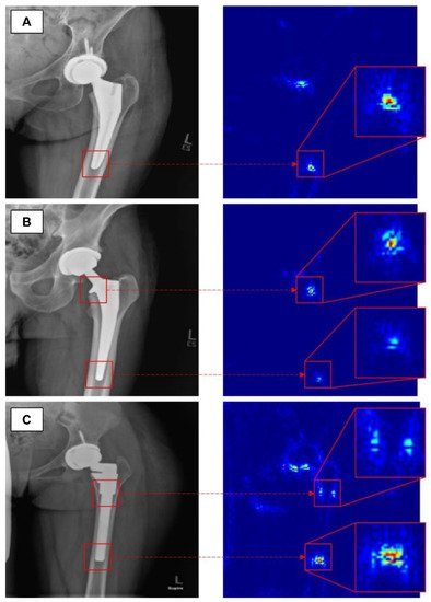
Advanced osteoarthritis of the hip or knee often requires arthroplasty. Several studies have introduced a model for classifying arthroplasty implants used by patients with deep learning algorithms. Karnuta et al. trained the InceptionV3 network-based CNN model using anteroposterior knee X-rays with nine different implant models inserted [33]. The trained model showed an accuracy of 99% and an AUC of 0.99, classifying the implant models at an almost perfect level. A similar attempt was made at the hip joint. In addition, Borjali et al. created a CNN model trained on 252 plain hip X-rays containing 3 different implant designs, and this model classified implants with 100% accuracy (Figure 2) [34]. Kang et al. also developed a CNN model trained on 170 plain hip X-rays containing 29 different implant designs. This model also showed a high level of performance, with an AUC of 0.99 [35].

Figure 2. The figure shows how a trained convolutional neural network classifies total hip replacement implants of different designs in A, B and C. Figure obtained from a study performed by Borjali et al. [34].
By contrast, the model classifying shoulder arthroplasty implants showed a relatively low AUC. Urban et al. developed a CNN model trained on 597 plain shoulder X-rays with 16 different implant designs, showing an accuracy of 80% [36]. In addition, Sultan et al. proposed a model for classifying the different designs of four manufacturers using modified ResNet and DenseNet, showing an accuracy of 85.9% [37].
In summary, as in the case of using deep learning for fractures, binary classification of osteoarthritis has a higher accuracy than multiclass classification. In particular, the CNN-based model for specifying arthroplasty implants of the hip or knee shows a high accuracy. This may be because, unlike human bone, the implant design is highly standardized, demonstrating a clear margin on X-rays and providing clear contrast information to the CNN model. However, the classification of shoulder arthroplasty implants shows a low level of accuracy. This may be due to the fact that a shoulder anteroposterior X-ray can show a wider range of positions than an anteroposterior radiograph of the knee or hip.
4. Deep Learning for Joint-Specific Soft Tissue Disease
As for deep learning approaches, an algorithm specialized for detection based on learned images and an algorithm for segmentation by analyzing features have structural differences and have developed into different areas of application [3]. In particular, segmentation has technical difficulties in that it is necessary to preserve spastic information that is easily lost in the outer-layer process of synthesizing the results of the CNN model being trained [38]. Recent studies have attempted to overcome these limitations through techniques such as FCN-based semantic segmentation.
These differences in deep learning algorithms also affect the use of deep learning in the orthopedic field. The deep learning-based studies introduced above are cases of diagnosing and classifying diseases based on X-ray images, and a CNN model specialized for segmentation is not always required [39]. By contrast, for diseases that are diagnosed and classified based on images such as ultrasound or MRI, a satisfactory level of accuracy can be obtained using only a CNN model specialized for segmentation. For example, a CNN model for diagnosing rotator cuff tears is more appropriate for inferring such tears based on the outline of the normal rotator cuff (segmentation) than a method of diagnosis applied by specifying the location where the tear occurred (regional detection).
Therefore, CNN models for diagnosing soft tissue disease in the orthopedic field have mainly been published after 2018, which was when the segmentation technology began to mature. Kim et al. trained a CNN model using a shoulder MRI dataset of 240 patients. The trained model identified the muscle region of the rotator cuff with an accuracy of 99.9% and graded fatty infiltration at a high level [40]. Taghizadeh et al. also conducted a similar study using a shoulder computed tomography of 103 patients as a dataset. The trained CNN model measured fatty infiltration with an accuracy of 91% [41].
Medina et al. introduced a model for segmenting the rotator cuff muscle with 98% accuracy by applying a CNN model trained using the shoulder MRIs of 258 patients [42]. Furthermore, Shim and Chung et al. introduced a model for evaluating the presence of tears and their sizes in the rotator cuff by training a Voxception-ResNet (VRN)-based CNN with 2124 shoulder MRIs. The trained CNN model diagnosed and classified rotator cuff tears with accuracies of 92.5% and 76.5%, respectively [10]. In addition, Lee et al. developed a new deep learning architecture using an integrated positive loss function and a pre-trained encoder. Using this, the location of the rotator cuff tear can be relatively accurately determined, even when imbalanced and noisy ultrasound images are provided [43].
Recent studies suggesting a CNN model for diagnosing meniscal tears, cartilage lesions and anterior cruciate ligament (ACL) ruptures in the knee joint have also been published. Couteaux et al. presented a model that trains a Mask-RCNN with 1828 T2-weighted 2D Fast Spin-Echo images to classify the torn part from the normal area of the meniscus and do so according to the location of the tear [44]. This model diagnosed and classified meniscal tears with an AUC of 0.91. Roblot et al. also proposed a model for diagnosing meniscal tears in a similar way, detecting meniscal tears with an AUC of 0.94 [45].
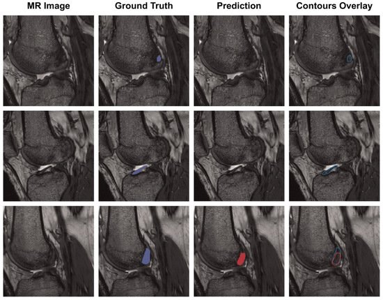
Chang et al. presented a model for diagnosing complete ACL tears by training a U-Net-based CNN using 320 coronal proton density-weighted 2D Fast Spin-Echo images, demonstrating an AUC of 0.97 [46]. In addition, Flannery et al. trained a modified U-Net-based CNN and evaluated the level of segmentation of the model. The segmentation level suggested by the trained model did not show a statistically significant difference from the ground truth (the value actually suggested by an expert) (Figure 3) [47].

Figure 3. Each row is the same MR slice, and each column is an unsegmented slice (MR Image), an expert measured value (Ground Truth), a trained CNN model predicted value (Prediction) and an overlay of manual and predicted segmentations (Contours Overlay). Figure obtained from a study performed by Flannery et al. [47].
This entry is adapted from the peer-reviewed paper 10.3390/app12020681
This entry is offline, you can click here to edit this entry!
