The first multi-cavity haloscopes for detection of dark matter axion in the RADES collaboration.
1. Background
Since Peccei and Queen established a mechanism to solve the strong Charge–Parity (CP) problem [1][2], and subsequently Weinberg [3] and Wilczek [4] predicted the existence of a new particle, the axion, the defining and execution of different experimental setups in order to detect this proposed particle have gained an increasing interest. In addition, soon after their proposal, axions were acknowledged to be ideal dark matter (DM) candidates, due to non-thermal production channels in the early Universe that are directly expected from the very Peccei–Quinn mechanism [5][6][7]. More recently, due in part to the persistently negative outcomes of the many worldwide efforts to detect weakly interacting massive particles (WIMPs), the favorite DM candidate for the last three decades, the axion DM hypothesis, has been attracting more interest in the experimental community.
2. First Multi-Cavity Haloscopes
2.1. All Inductive 5-Cavity Haloscope
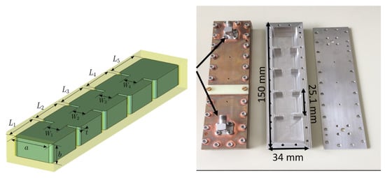
During 2017, the first RADES haloscope was designed, manufactured, characterized, and finally used in the 2018 data-taking campaign in CAST. It was the fivefold cavity shown in
Figure 1 and presented in
[8]. Dimensions, as described in
Figure 1.
Figure 1. RADES 5-cavity haloscope: scheme and dimensions, and device before copper plating.
This device was designed first through the formalism in
[8], and was finally optimized with CST Studio
[9].
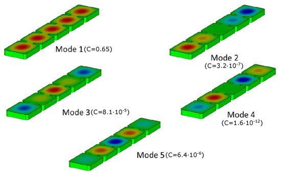
Figure 2 shows the five different configurations of the mode
 TE10
TE10for the final five-cavity structure, and the corresponding form factors.
Figure 2. Electric field pattern (vertical polarization) for the five different configurations of mode TE101
for the 5-cavity haloscope, with the associated form factors. The red fields denote positive levels, the green fields zero, and the blue fields negative. Taken and modified from
[8].
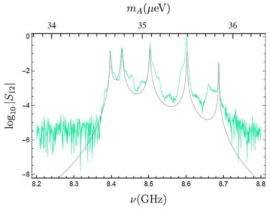
Occasional quenches produced in the CAST magnet made necessary a strong material for the haloscope in order to avoid deformations in the device. For that reason, the base material was not copper, but non-magnetic stainless steel 316LN, plated with a 30 μm of copper layer for reducing the losses. The transmission coefficient magnitude, both simulated and measured at the operation temperature of 2 K, is depicted in Figure 3.
Figure 3. Transmission coefficient magnitude at 2 K: simulated (black) and measured (green), where measurements include the effects of cables from and to the VNA. Taken and modified from
[8].
2.2. Alternate Coupling
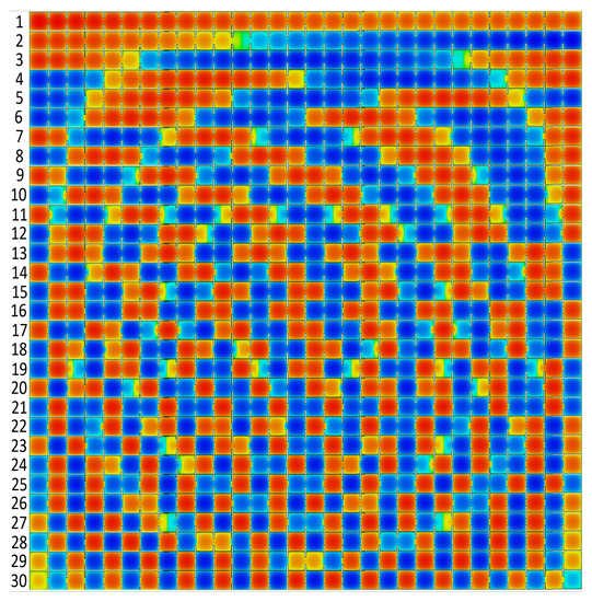
Although the multicavity concept alleviates the mode clustering, it has also a limit. N cavities produce N different configuration patterns for TE101TE101
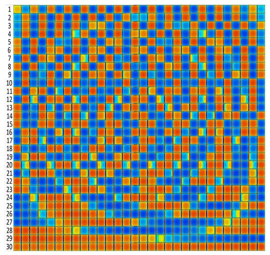
mode. Therefore, when the number of cavities increases, the same concentration of resonances is observed. Figure 4 shows the 30 configurations of a 30-cavity haloscope with a similar design to the 5-cavity one, i.e., inductive irises. Figure 5 shows the spectrum of this device with these resonances.
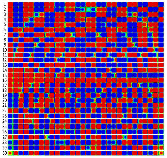
Figure 4. Electric field pattern (vertical polarization) for the thirty different configurations of mode TE101 TE101
for the all-inductive 30-cavites haloscope. Numbers on left side refer to the order of the configuration resonances with the frequency. The red regions denote positive E-fields, and the blue regions negative ones.
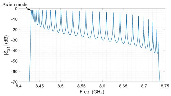
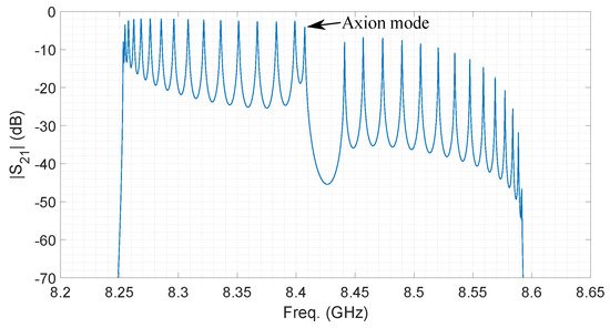
Figure 5. Simulated transmission coefficient magnitude of an all-inductive 30-cavity haloscope at 2 K.
As observed, the first (axion one) and the second TE101TE101
mode configurations are very similar. This situation worsens with the manufactured device and data-taking conditions, leading normally to an overlapping of both resonances, which makes it impossible to obtain the quality factor or the coupling factor from measurements.
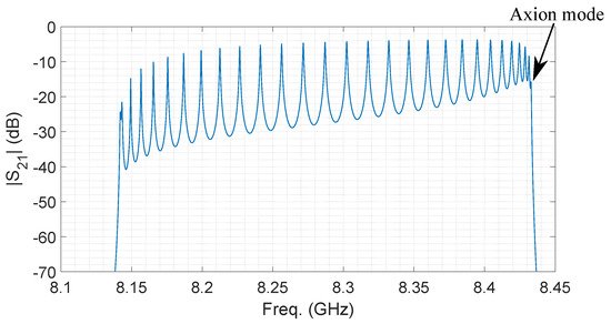
For an all-capacitive coupling, the patterns and spectrum are shown in Figure 6 and Figure 7, respectively. In both spectrums, thirty modes can be seen (not by eye due to numerical accuracy from the software). However, there is a main difference between them: for the all-inductive structure, the axion mode is the first peak, whereas for the all-capacitive structure, the axion mode is the last one (30th mode). Note that in both cases, the axion mode is at the same frequency (∼8.43 GHz). The reason comes from the design parameters employed to set such an axion search at that specific frequency.
Figure 6. Electric field pattern (vertical polarization) for the thirty different configurations of mode TE101 TE101
along the all-capacitive 30-cavites haloscope. Numbers on the left side refer to the order of the configuration resonances with the frequency. The red regions denote positive E-fields, and the blue regions negative ones.
Figure 7. Simulated transmission coefficient magnitude of an all-capacitive 30-cavity haloscope at 2 K.
The solution to avoid the mode-mixing close to the axion mode is to apply alternated couplings: capacitive + inductive irises
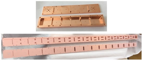
[10]. In this configuration the axion mode is at the middle of the band, where greater mode separation exists. The first haloscope designed and manufactured with this alternating concept was a 6-cavity structure (
Figure 8 (top)), followed by a 30-cavity structure based on the same idea (
Figure 8 (bottom)).
Figure 9 shows the thirty E-field patterns of this last haloscope, the sixteenth configuration being the most adequate for the axion–photon coupling, that is, with maximum form factor. The spectrum of this structure in the frequency range of interest is shown in
Figure 10, where an improvement regarding the mode-mixing can be observed. Concretely, the alternate coupling allows a 32-fold greater separation between the axion mode and the closest neighbor.
Figure 8. Manufactured 6cav and 30cav structures with alternated couplings.
Figure 9. Electric field pattern (vertical polarization) for the thirty different configurations of mode TE101 TE101
for the alternating 30-cavites haloscope. Numbers on the left refer to the order of the configuration resonances with the frequency. The red regions denote positive E-fields, and the blue regions negative ones.
Figure 10. Simulated transmission coefficient magnitude of an alternating 30-cavity haloscope at 2 K.
This entry is adapted from the peer-reviewed paper 10.3390/universe8010005