Classical Guitar Modelling Technologies

Classical Guitar Modelling Technologies: History

Please note this is an old version of this entry, which may differ significantly from the current revision.

Subjects: Engineering, Mechanical

Contributor: Alexandre Marks Löw , César Vasques

Due to the diversity of phenomena involved in the modeling of musical instruments and the inherent difficulties in formulating vibroacoustics problems, including the various underlying possible dissipating effects, and despite the availability of some classical and computational approaches, this task remains a significant challenge after many years. Analytical modeling and numerical simulation of multiphysics coupled systems is an exciting research area, even when it comes to intrinsically linear or linearized formulations, as is usually the case with coupled vibroacoustic problems. The combined effect of many localized geometrical miss-modeling with significant uncertainty in mechanical characterization of some organic materials yields large discrepancies in the natural frequencies and mode shapes thus obtained.

classical guitar
lumped-parameter modeling
finite element method
vibroacoustics
frequency domain
musical instruments
luthiery

1. Simplified Guitar Models

1.1. Formulation of Simplified Models and Definition of Parameters

In what follows, the equations of simplified 2 and 3 DOF models for low frequency vibro-acoustic response of the resonant chamber (guitar body) will be presented, trying to keep clarity and conciseness as possible. The meaning of each index adopted in the development of the equations below is shown in Table 1 (for an explanation of guitar components, refer to Figure 1 below). Table 2 presents the parameters appearing in the equations of the 4 DOF model ^[1]; it should be noted that those appearing in the equations for 2 and 3 DOF models ^[2]^[3]^[4] are also covered in this table, but some table entries do not apply for the simpler models. Damping coefficients are presented separately on the last line because these parameters are to be defined through experimental modal analysis.

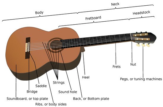
Figure 1. Acoustic guitar parts. (Source: adapted from original image due to William Crochot, distributed under CC BY-SA 3.0 license; Wikimedia Commons).

Table 1. Meaning of the indexes used in the various vibroacoustic models of the classic guitar.

Index	Meaning
t	Top plate
a	Air column through the sound hole
b	Back plate
r	Ribs (i.e., the remaining parts moving as a whole)

Table 2. Equivalent parameters of all 3 models and damping coefficients.

Symbol	Description	Units
V	Air volume inside the resonant chamber	$m^{3}$
$m_{a}$	Equivalent mass of the air column	$kg$
$m_{t}$	Equivalent mass of the top plate	$kg$
$m_{b}$	Equivalent mass of the back plate	$kg$
$m_{r}$	Equivalent mass of the ribs	$kg$
$A_{a}$	Equivalent area of the air column	$m^{2}$
$A_{t}$	Equivalent area of the top plate	$m^{2}$
$A_{b}$	Equivalent area of the back plate	$m^{2}$
$k_{t}$	Equivalent stiffness of the top plate	$N / m$
$k_{b}$	Equivalent stiffness of the back plate	$N / m$
$ζ_{i}$ , $η_{i}$	i-th mode damping coefficient $(i = 1, \dots, 4)$	−

About the damping parameters in Table 2, it is important to emphasize at this point that these coefficients alone would imply, for instance, a purely viscous, or viscoelastic/hysteretic dissipation behaviour, which is clearly a non-physical assumption considering the predicted forms of energy loss in the modelling of vibro-acoustic coupled systems; i.e., the energy balance in this cases should include, at least, some sort of viscous, viscoelastic and acoustic radiation forms of damping ^[5]^[6]. Indeed, for those parameters related to energy dissipation, that equivalent modelling approach mentioned earlier is almost always adopted—with damping ratios, loss factors or another dissipation quantifier accounting alone for all forms of energy loss.

1.1.1. Simplified 2 Degrees-of-Freedom Model

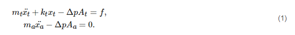
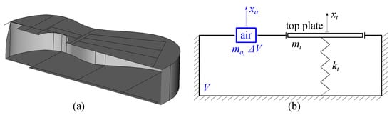
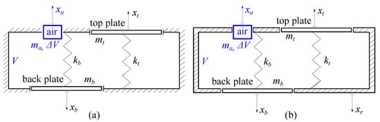
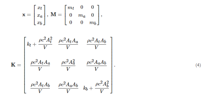
Now, suppose the tensions in guitar strings transmit a force of magnitude f through the bridge (see Figure 1), that can be represented as acting pointwise, up and down, in the centroid of top plate. Thus, the equations of motion representing the dynamic coupling with the air column DOF displayed in Figure 2 can be written as

Figure 2. Schematic of the simple 2 DOF model: (a) Cut plane view of a guitar resonant chamber 3D CAD model, constructed with shells, planes and lines for subsequent FE analysis. (b) Representation as a simple 2 DOF model, considering only the motion of top plate and air column.

Considering the adiabatic, linearized form, of the equations of acoustics, the pressure variation

Δ p

may be expressed in terms of the total volume V inside the resonant chamber, the sound velocity c and mass density

ρ

of the surrounding air, and of the (idealized) chamber volume increment

Δ V = A_{t} x_{t} + A_{a} x_{a}

^[7], as

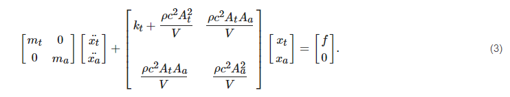
Thus, substituting Equation (2) into (1) and writing it in matrix form, i.e.,

M \ddot{x} + K x = f

, yields

Quantities appearing on the left-hand side of Equation (3) could be viewed separately into two classes: those described in Table 2 depend on geometric and/or material properties of guitar components, and thus shall be treated as adjustable parameters of the equivalent system, while the remaining ones (speed of sound and mass density) are physical properties of the surrounding air, and so it is more reasonable to consider them as system-independent constants. On the other hand, the driving force f would be truly impossible to obtain, both experimentally or analytically, because this excitation motion is rather imposed by an effectively distributed conjugate on the interfacing area between the top plate and the bridge; i.e., its much higher stiffness impels it to rotate when forced to and fro by the tension of guitar strings, acting some distance above the plate. Theoretically, once the plate is adequately approximated (to some level of accuracy) as a clamped or hinged plate ^[1] an equivalent pivot distance could be considered, via static equilibrium of moments, in order to compare the driving force over the top plate with the tension in guitar strings. This approach has not been explored up to this moment, however, to the authors’ knowledge. Nevertheless, analytical values for modal parameters can be readily extracted from this matrix equation, and in this way it has been extensively used for model comparison ^[8]^[2]^[9], structural modifications prediction based on eigenvalues sensitivity ^[9]^[4] or frequency domain model updating ^[10].

Unlike the mentioned references, the previous equations were written in undamped form. While this choice was made primarily to simplify the presentation, it has a more profound justification stemming from the authors’ previous works ^[11] that is: given the levels of uncertainty in these simplified models, the use of more complex, non-proportional damping formulations would not cause any perceivable alteration in measurable outputs. Thus, since a proportionally damped analytical system produces the same eigenproperties as its undamped version, and taking into consideration the prominence of modal parameters over the forced response for the envisaged applications, damping factors can be confidently considered here as fine tuning adjustments. Among the myriad of available methods to extract damping coefficients (along with mode shapes and natural frequencies) from measured responses, Subspace-Stochastic Identification (SSI) has proven to be a very convenient, output-only, alternative ^[11].

1.1.2. Simplified 3 and 4 Degrees-of-Freedom Models

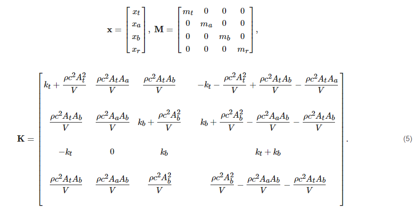
From the definitions presented above for 2 DOF, modelling extensions can be readily devised. Figure 3 shows schematic representations for two of these possible expansions, resulting in 3 and 4 DOF models, respectively. The most obvious approach then is to consider the flexibility of back plate in a symmetrical manner as was made for the top plate. This in turn adds up three more free parameters: the mass, the stiffness and one more modal damping coefficient, and the system can now vibrate with three linearly independent modes. Thus, following ^[4], the resultant displacements vector and the corresponding mass and stiffness matrices for the 3 DOF model are given as

Figure 3. Schematic of 3 and 4 DOF simplified models; (a) 3 DOF: allowing for motions on top and back plates, and air column through the hole. (b) 4 DOF: basically allowing for the same motions of the 3 DOF model, plus one for the entire structure (free condition).

The next modeling extension, considering mass and motion for the ribs, is a little bit trickier and thus needs deeper attention. First of all, the motion allowed for the ’ribs’ in fact means that the whole guitar is free to move. Thus, this is not exactly about freeing a motion in the same sense as it was done for the back plate, but rather allowing a fully free boundary condition. As the governing equations of the 4 DOF model in ^[1] are not explicitly presented in matrix form, the resulting stiffness matrix for this model was derived, and is written below as

2. Finite Element Modelling of Acoustic Guitar Vibroacoustics

Many factors have contributed to the popularity of FE modelling in the last two or three decades, but most of all, possibly, the greater availability of computational resources. Thus, it is not surprising that nowadays, the bulk of academic research in vibro-acoustics of musical instruments makes use of it to a greater or lesser extent. In what follows, a literature survey on succesful applications of FE modelling for coupled simulation of acoustic guitar is presented. Brooke ^[12] was a pioneering work on the application of FE to guitar coupled vibro-acoustics. The simplified models were employed alongside the FE modelling of the top plate and boundary element (BE) model of surrounding air, thus achieving an organic coupling between lumped parameters and domain discretization approaches. Elejabarrieta, Ezcurra and Santamaría ^[13]^[14] performed fluid-structure interaction FE analyses, both for fluid and structural domains. The fluid domain was considered only in a small air column, in a similar fashion as was done for the lumped models discussed earlier. Neck and headstock participations were disregarded. 8474 brick elements were used to model the structure, while the mesh on the fluid domain was adjusted to give sufficiently accurate results up to 1 kHz. Comparison of coupled and uncoupled mode shapes confirmed the physical insights brought by lumped models and the importance of Helmholtz frequency to the lower range coupled dynamics. Chaigne and collaborators ^[15]^[16]^[17] successfully employed FE and finite differences in a full non-linear transient simulation, where considerable effort is put into precise definition of purely mathematical aspects related to the problem’s well-posedness and stability of the proposed solution procedure. The fictitious domain method was used to avoid what they called an ‘ectoplasm’, referring to the rather artificial definition of boundaries in the fluid domain. Structural flexibility of the resonant chamber is considered only within the top plate, disregarding fan bracing. Both these simplifications may leave aside important aspects of top plate dynamic behaviour. It is interesting to note that, despite the clear relevance of such a complete description, these important features are especially focused on by the lumped-parameter models presented above. Other instruments, closely related to the acoustic guitar, were successfully modelled via FE analysis as well, and we pinpoint here references ^[18], on the Brazilian viola caipira, and ^[19], on the Colombian bandola.

This entry is adapted from the peer-reviewed paper 10.3390/ASEC2021-11179

References

Popp, J.E. Four mass coupled oscillator guitar model. J. Acoust. Soc. Am. 2012, 131, 829–836.
Christensen, O.; Vistisen, B.B. Simple model for low-frequency guitar function. J. Acoust. Soc. Am. 1980, 68, 758–766.
Caldersmith, G. Fundamental coupling and its musical importance. Catgut. Acoust. Soc. Newsl. 1981, 36, 21–27.
French, R.M. Engineering the Guitar: Theory and Practice; Springer: New York, NY, USA, 2008.
Gaul, L. Tutorial Guideline VDI 3830: Damping of Materials and Members. In Modal Analysis Topics, Volume 3, Proceedings of the 29th IMAC, Jacksonville, FL, USA, 31 January–3 February 2011; Springer: New York, NY, USA, 2011; pp. 17–25.
Cremer, L.; Heckl, M. Structure-Borne Sound: Structural vibrations and Sound Radiation at Audio Frequencies; Springer: Berlin, Germany, 1973.
Pierce, A.D. Acoustics—An Introduction to Its Physical Principles and Applications, 3rd ed.; Acoustical Society of America: Melville, NY, USA, 1989.
Caldersmith, G. Guitar as a reflex enclosure. J. Acoust. Soc. Am. 1978, 63, 1566–1575.
French, R.M. Structural modification of stringed instruments. Mech. Syst. Sign. Proc. 2007, 21, 98–107.
Löw, A.M. Identificação Modal Experimental da Caixa Acústica de um Violão Clássico. Master Thesis, Universidade Federal do Rio Grande do Sul, Porto Alegre, Brasil, 2012. (In Portuguese).
Löw, A.M.; Gomes, H.M.; Prado, G.S.; Vasques, C.M.A. A Generalized Proportional Damping Model Applied to a Guitar Model. In Proceedings of the 25th International Congress of Mechanical Engineering, Uberlândia, Brasil, 20–25 October 2019.
Brooke, M. Numerical Simulation of Guitar Radiation Fields Using the Boundary Element Method. Ph.D. Thesis, University of Wales, Cardiff, Wales, 1992.
Elejabarrieta, M.J.; Ezcurra, A.; Santamaría, C. Coupled modes of the resonance box of the guitar. J. Acoust. Soc. Am. 2002, 131, 829–836.
Ezcurra, A.; Elejabarrieta, M.J.; Santamaría, C. Fluid-structure coupling in the guitar box: Numerical and experimental comparative study. Appl. Acoust. 2005, 66, 411–425.
Derveaux, G.; Chaigne, A.; Joly, P.; Becache, E. Time-domain simulation of a guitar: Model and method. J. Acoust. Soc. Am. 2003, 114, 107–126.
Becache, E.; Chaigne, A.; Derveaux, G.; Joly, P. Numerical simulation of a guitar. Comput. Struct. 2005, 83, 3368–3383.
Chaigne, A.; Kergomard, J. Acoustics of Musical Instruments; Springer: New York, NY, USA, 2016.
Paiva, G.O. Análise Modal Vibroacústica da Caixa de Ressonância de uma Viola Caipira. Master Thesis, Universidade Estadual de Campinas, Campinas, Brasil, 2013. (In Portuguese).
Rodríguez, S.E. Numerical Analysis of the Modal Coupling at Low Resonances in a Colombian Andean Bandola in C Using the Finite Element Method; Undergraduate Report; Universidad EAFIT: Medellín, Colombia, 2012.

© Text is available under the terms and conditions of the Creative Commons Attribution (CC BY) license; additional terms may apply. By using this site, you agree to the Terms and Conditions and Privacy Policy.