Mathematical Background of 5D model of the aorta

Mathematical Background of 5D model of the aorta: History

Please note this is an old version of this entry, which may differ significantly from the current revision.

Subjects: Engineering, Biomedical | Health Care Sciences & Services | Mathematics, Applied

Contributor:

Visualization is crucial for the display and understanding of medical image data. For diagnostic and surgical planning, radiologists and surgeons must be able to evaluate the data appropriately. Many imaging systems’ data can incorporate both functional and structural information, resulting in 4D datasets. When the image contains spectral information, it can be extended to 5D in some circumstances. Overall, 5D imaging reveals more information than 4D imaging.

5D model of the aorta
ﬂuid solver
pressure
ﬂow rate
Reynolds number
velocity
MRI

1. Dynamics of Laminar Viscous: Navier-Stokes Equations

Fluid flow simulations are based on Newtonian and fluid property physics. Physical rules, such as the maintenance of kinetic energy, which contribute to the equation of motion, must be satisfied by these features. The viscous stress tensor is linearly related to the rate of the strain tensor in a Newtonian fluid. Assume Stokes flows (low Reynolds number) and only slight spatial variations in hydrostatic pressure [21].

Let Ω ⊂ R2 be an open domain bounded and connected to the Lipschitz boundary Γ. Consider the Navier–Stokes equation

\partial v \partial t - ν d i v (\nabla v + (\nabla v) T) + (v \cdot \nabla) v + \nabla p = f i n Ω

(1)

div v = 0 i n Ω

(2)

With the initial condition v (0) = v0, where v is the velocity, p is the pressure, ν is the viscosity (or the inverse of the Reynolds number, i.e., ν = 1(/Re)), it is an external time-dependent body force when the Reynolds number approaches a critical value or minor fluctuations are implemented into the flow. It is well understood that the flow transitions from laminar to turbulent [22].

The fluid was intended to be incompressible in this simulation, which meant that the density had to be steady and Newtonian. The vessel wall had to be impervious to deformation. A volumetric flow waveform was defined at the inlet of the pulsatile flow. For the entry of this model, a fully defined laminar velocity profile was used. The blood fluid was set to have a density of 1056 (kg/m³) and a viscosity of 0.06 (Pa. These fluid properties set the Womersley parameter (α), which measures the frequency of the pulsation, defined as [23]:

α = D ( ω υ ) - 0.5 2

(3)

where ω is the angular frequency, and υ is the kinematic viscosity of the fluid. Properties of the fluids are mentioned for this model as well as the boundary conditions.

In laminar flow regimes, the related term of the Navier–Stokes equation can be used to measure the volume of the viscous dissipation process [20]

Φ v D = 1 2 μ Σ i Σ j [(\partial v \partial x i + \partial v \partial x j) - 2 3 (Δ - ν) δ i j] 2

(4)

where Φ_vD is the viscous dissipation per unit volume based on the viscous dissipation term, and μ is the dynamic viscosity. δij = 1 for i¼j and δij = 0 for i ≠ j, where i and j are the principal directions (x, y, z) in Equation (4), which consists of the elastic viscosity of the velocity field and the spatial derivatives. If the speed field is defined, such as from 4D flux MRI measurements, Equation (4) can be used to quantify the viscous dissipation per unit volume. The integral of the viscous dissipation of the unit was used to measure the overall viscous dissipation.

\int Φ v D d v = Σ n u m v o x e l s i - 1 Φ v D v i

(5)

2. Boundary Conditions

The condition was extended to the fluid model, and the vessel walls were considered to have a slip-resistant boundary. The porosity of vessels is often underestimated. As a result, the fluid is not supposed to move through the vessel walls as it passes through it. The boundary conditions applied to the vessel walls are [23]:

u i = u j = 0

(6)

There must be no increase in velocity in the steering radial along the line’s equatorial plane, essentially reducing the radial portion of the velocity to zero. Consequently, the applied boundary condition is

u i = \partial u i \partial x i = 0

(7)

The incompressible Newton flow rate through the established geometry is depicted by a parabolic velocity profile. As the Dirichlet boundary state at the output, a variable and spatially uniform pressure boundary condition is applied, and for the limit condition, the velocity Neumann (zero gradient of velocity in the axial direction at the output) is applied [24].

The wall of the aorta was rigid. Consequently, the walls of the flow domains were static and stationary. Boundary conditions for speed were imposed on the wall with no slip or flow. The non-flow condition means that the velocity in the normal direction of the wall is zero because the walls are impervious. The pressure gradient perpendicular to the wall was considered negligible using the Navier–Stokes equations [25].

Blood is a vigorous medium because its viscosity varies as a feature of the shear deformation rate, making it behave like a non-Newtonian fluid. Blood is biologically smoother in the systolic crest than when it moves slowly, as in the diastolic crest. This occurs as red blood cells clump together. The impact of thinning blood shear is as follows [16,23]:

μ (γ) = μ x + μ 0 - μ x ( 1 + m γ ) a

(8)

In this equation,

μ_{0}

is the viscosity of blood at zero strain rates, and

μ_{\infty}

is the viscosity of the blood at an infinite or very high strain rate. The constants m, n, and a were experimentally determined.

3. Characteristics of Blood Flow Fluids

3.1. Blood Viscosity, μ

The sensitivity of a fluid to deformation under shear stress is known as viscosity. This is a type of fluid “friction”, which explains the internal resistance of the fluid to the flow. The viscosity of a fluid is strongly influenced by the bonds between the molecules. The viscosity is mathematically defined as the ratio of the shear stress to the velocity gradient. The majority of fluids are Newtonian fluids, which have a steady viscosity. Plasma, blood cells, and other substances carried in the blood make up the blood. The number of particles in the plasma induces non-Newtonian activity in the blood, which means that the viscosity varies with the flow shear rate. The blood flow exhibits Newtonian flow behavior when the shear rate is sufficiently high. In normal situations, however, it is not possible to disregard the fluid’s non-Newtonian behavior [26].

3.2. Geometry Design

In the “no fall” condition placed at the boundary, fluid in contact with the vascular wall can pass at the same pace as the wall. This is because the shear forces imposed by the wall on the fluid will ultimately cause the boundary flow to have the same velocity as the downstream surface, which is a rational statement in this analysis. Meanwhile, to preserve mass equilibrium, the flow away from the vessel wall continues to speed up until it reaches an established profile, where no further velocity profile changes occur in the flow direction. This causes a non-zero speed gradient,

\frac{\partial y}{\partial u}

, where u and y are the velocity component in the direction of flow and the coordinate of the space perpendicular to the direction of flow, as shown in Figure 1.

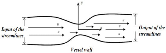
Figure 1. Modeling of the stenosing aorta.

Mathematical relationship between shear stress of the wall, τ, and viscosity, μ blood, as explained in Section 2.3.1, is indicated in Equation (8) [23]:

τ = μ \partial y \partial u

(9)

It was shown that achieving this quantity using experimental methods and relying on the experience of the fluid’s viscosity and velocity profile near the vessel wall is challenging. This sum is easier to approximate using CFD techniques, but it is based on mesh consistency.

The governing equations for simulating the hydrodynamic flow of blood through a stenosing aorta with sufficient boundary conditions are as follows [16]:

\partial u i \partial x i = 0

(10)

Laminar pulsed flows describe the boundary conditions at the entrance of the stenosing aorta. Because all of the geometries’ inputs are circular, a speed limit is enforced to introduce spatial and temporal differences in the pulsed flow. Patients with aortic stenosis are most likely to have valvular stenosis. This study aimed to determine the effect of physiological conditions on the rupture wall of the stenosing artery.

3.3. Reynold Number

Laminar and turbulent flows are the two main types of flows that arise. Turbulence is a measure of the degree of oscillation of the surrounding fluid in the direction normal to the fluid flow, and it can be made on the basis of both the energy (kinetic energy of turbulence) and energy dissipation (dissipation turbulence rate) included in this motion. There is also little distinction between laminar and turbulent flows in terms of fluid particles. In chaotic flows, the particles appear to behave spontaneously, which is similar to the initial flow direction on average. The average fluid velocity, density, viscosity, and vessel diameter all play a role in determining when the fluids become turbulent (for internal flows). The Reynolds number Re is the name given to this characteristic value, as shown in Equation (12):

R e = U D v = ρ U D μ

(11)

where U is the average velocity of the fluid, D is the diameter of the vessel, ρ is the density of the fluid, μ is the fluid viscosity (dynamic), and ν is the kinematic viscosity of the fluid. The fluid tends to become turbulent at a Reynolds number of approximately 2000 for internal flows [27].

The laminar and turbulent flows have different profiles, as shown in Figure 2.

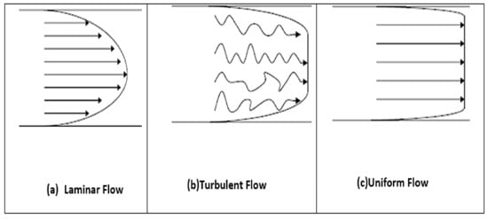
Figure 2. Velocity profiles for laminar (a), turbulent (b) and uniform (c) flow [9].

It is extremely unlikely that blood can enter turbulent flow under natural circulation conditions. Only severely stenosed vessels, extremely abnormal flow paths, and even certain pathological disorders that impair blood flow properties cause this. Non-Newtonian fluids have a flatter profile toward the axes, so the formed profiles are different. Blood appears to have a uniform velocity profile rather than a developed profile because of the diverse flow paths and irregular sizes of arteries [28,29].

3.4. Assessment of the Rate of Severe Stenosis

The amount of cross section that is “blocked” by occlusion determines the degree of stenosis. The narrowest segment (called “groove”) of the blockage is usually considered the cross section for stenoses with variable geometry. Figure 3 depicts a common model of a tube with a single stenosis in which the original radius of the vessel R0 is obstructed by a stenosis with a normalized maximum height of value = h/R₀, where h is the maximum height of the stenosis. To obtain the unit length, the available radius, R₀ = 1. Because the standardized height of the stenosis must be 0 ≤ δ <1, we can deduce the following [23].

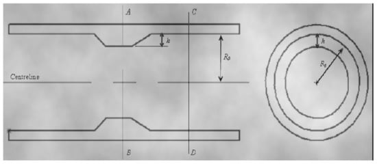
Figure 3. The geometry showing the height of the stenosis, δ, initial radius of the vessel, R₀ [9].

The normalized cross section of light through CD = π

The normalized cross-section of light on AB = π (1 − δ) 2

Thus, the percentage of blocked area can be derived; therefore, the severity of the stenosis is obtained as follows:

π - π [ 1 - δ ] 2 π \times 100 % = (1 - [1 - δ] 2) \times 100 %

(12)

This entry is adapted from the peer-reviewed paper 10.3390/biomedinformatics2010002

© Text is available under the terms and conditions of the Creative Commons Attribution (CC BY) license; additional terms may apply. By using this site, you agree to the Terms and Conditions and Privacy Policy.