Your browser does not fully support modern features. Please upgrade for a smoother experience.
Please note this is an old version of this entry, which may differ significantly from the current revision.
Magnetic resonance imaging (MRI) is a technique for mapping the interior structure of the body as well as specific aspects of functioning.
- deep learning
- transfer learning
- ResNet50
- convolutional neural networks
- magnetic resonance imaging
- MRNet
1. Introduction
The application of artificial intelligence in the healthcare industry has grown substantially in recent years [1] since it may enhance diagnostic accuracy, boost efficiency in workflow and operations, and make monitoring of the patient’s suffering easier. In the healthcare industry, computer-based technology is provided through collecting digitised data in fields [2], such as computed tomography (CT) [3], magnetic resonance imaging (MRI), X-ray [4], and ultrasound [5,6]. However, most of the best examples of the high performance of deep learning are in the field of computer vision by examining medical images and videos [7]. With breakthroughs in deep learning and image processing [8,9], it has the potential to recognise and locate complex patterns from several radiological imaging modalities, many of which even have recently demonstrated performance comparable to human decision making [1]. When reading medical images, radiologists frequently scan the entire image to locate lesions, analyse and quantify their attributes, and then define them in the report. This normal procedure takes a long time. More critically, certain important abnormal outcomes may go unnoticed by human readers [1]. Technological advancements have made it possible to generate high-resolution magnetic resonance (MR) images in a short amount of time, allowing for faster scanning. The employment of deep learning approaches to diagnose utilising MRI data from diverse parts of the body is very common [10,11,12,13].
The MR image is produced by keeping the patient inside a gigantic magnet that induces a relatively powerful external magnetic field [14]. Geometric planes used to section the body into pieces are called body planes. They are commonly used to define the placement or orientation of bodily structures in both human and animal anatomy. Anatomical terminology refers to reference planes as standard planes. The body is divided into dorsal and ventral portions by the coronal plane (front or Y-X plane). The axial plane (axial or X-Z plane) divides the body into superior and inferior (head and tail) portions. It is usually a horizontal plane that is parallel to the ground and runs through the centre of the body. The sagittal plane (lateral or Y-Z plane) divides the body into sinister and dexter sides [15]. Figure 1 shows these axes.
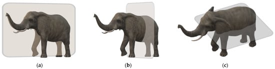
Figure 1. (a) Sagittal plane; (b) coronal plane; (c) axial plane [16].
2. Selecting Eligible Data
The adoption of standardised datasets and benchmarks for assessing machine learning algorithms has been a crucial factor in the advancement of computer vision. The scope of the tasks being addressed is defined by these datasets, which frequently include imaging data with human comments [7]. Transfer learning aims to maximise learning performance in the targeted field by storing acquired knowledge while addressing a problem and then transferring that knowledge that has been found in different but related fields. This may make it possible to avert the necessity for a large amount of data for the field targeted to be trained [39]. ImageNet [40] is a high-profile example of a large imaging dataset utilised to benchmark and examine the relative performance of machine learning models in the still image dataset field [41].
When examining the studies on modern convolutional neural networks, LeNet [42], developed by LeCun et al. in 1998; AlexNet [31], created by Krizkevsky et al. in 2012; VGGNet [43], produced by Simonyan and Zisserman at the Visual Geometry Group (VGG) laboratory in 2014; and residual networks (ResNet), built by He et al. in 2015, can be cited. Prior to ResNet, it was believed that increasing the number of convolutional layers would enhance the performance rate. On the contrary, increasing the network depth led to the vanishing gradient problem. The vanishing gradient issue appears when the impact of the initial layers is considerably weakened during backpropagation since the impact of the multipliers is drastically diminished. This problem is addressed by establishing shortcut connections between layers in the ResNet model. The vanishing gradient problem is handled by using these shortcuts to transfer the gradient values in the model after the residual blocks.
Multiple images are added one after the other to make up the MRI data. Selecting the eligible images to diagnose the disease while working on these images will improve the efficiency of the study. In addition, the accuracy of the classification process was checked, and the diagnosis of over noisy and damaged images were identified while selecting the eligible images.
3. Selecting the Relevant Area
Selecting the relevant regions would improve the accuracy of the study by focusing on the region where the disease will be diagnosed rather than looking at the entire image during the diagnostic phase. The study by Saygılı et al. [50] aimed to search the meniscus structures in a completely narrowed area with regard to this, which they performed by manually marking the MR images. They analysed a dataset that included both healthy and unhealthy MR images with varying degrees of discomfort. The dataset they employed contained 88 MR images that were labelled by radiologists. The study investigated the effect of feature extraction methods of histograms of oriented gradients (HOG) [51] and local binary pattern (LBP) [52]. HOG and LBP are feature extraction methodologies that produce successful results. HOG is a feature extraction methodology that delivers accomplished image recognition results. In this method, the feature is extracted with the gradients and orientations of the pixels on the image.
The ResNet50 model, which was pre-trained through ImageNet, is suitable for working with three-channel images [44]. The images in the MRNet dataset have the sizes 256 × 256 × 1. Therefore, one-channel images must be converted to three-channel ones. During this conversion, a function was built to convert all the images into three-channel images. Every time a new one-channel visual arrives at a function, the colour value of each pixel is repeated three times in an empty matrix of 256 × 256 × 3 dimensions within the function to generate a new image, according to the working logic of the function. Figure 2 demonstrates the conversion of a one-channel image to a three-channel.
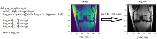
Figure 2. The function used to increase the number of channels and, an example of a 256 × 256 × 1 coronal image, which was converted to 256 × 256 × 3.
The exponential decay learning rate was employed to develop a learning rate that drops as the training progresses. The initial learning rate was initially set at 0.01 and declined with a decay rate of 0.96 at 4000 decay steps. Stochastic gradient descent (SGD) was used as the optimiser. It is known that SGD has large oscillations [45]. Li et al. [46], on the other hand, demonstrated the SGD oscillation variation when the exponential decay is employed and utilised with different momentum values. Figure 3 shows the model’s structure as well as its parameter values.
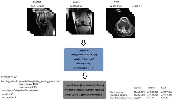
Figure 3. General structure of image classification model.
Figure 4a depicts the classification of images pertaining to a patient in a classification process; Figure 4b shows the confusion matrix produced after the training of sagittal images as a result of the data classification test of 10 patients, while Figure 4c provides the accuracy of 40 epochs and Figure 4d gives the train and validation loss values.
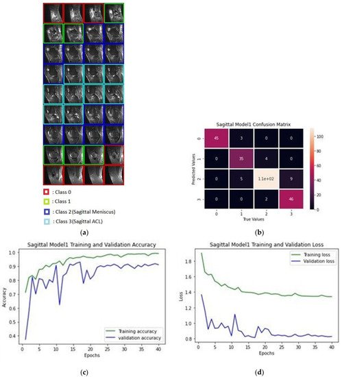
Figure 4. (a) Classification process of sagittal MRI; (b) confusion matrix of the produced validation dataset for sagittal plane; (c) training and validation accuracy rates; (d) training and validation loss values.
Upon the examination of sagittal train and valid images, six trains and two valid data appeared to be not selected. The unselected images were observed to be misclassified and over noisy images. Table 2 contains a list of unselected images, and Figure 5 shows one example of unselected images.
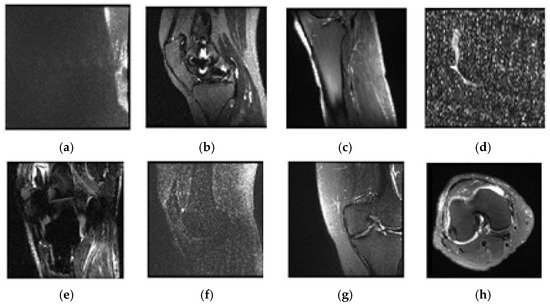
Figure 5. Examples of unselected images and patients’ numbers in the dataset: (a) 0003; (b) 0370; (c) 0544; (d) 0582; (e) 0665; (f) 0776; (g) 1159; (h) 1230.
This entry is adapted from the peer-reviewed paper 10.3390/make3040050
This entry is offline, you can click here to edit this entry!