Deep learning gained popularity during the last decade [26,27,28]. Convolutional neural networks have been widely used in the classification of diseases [29,30]. It is challenging to train a CNN architecture if the datasets have a limited number of training samples. In [18], a partial transferable CNN was proposed in order to cope with a new dataset with a different spatial resolution, a different number of bands, and variation in the signal-to-noise ratio. The experimental results using different state-of-the-art models show that partial CNN transfer with even-numbered layers provides better mapping accuracy for the target dataset with a limited number of training samples. In [19], a novel method using transfer learning to deal with multi-resolution images from various sensors via CNN is proposed. CNN trained for a typical image data set, and the trained weights were transferred to other data sets of different resolutions. Initially, skin cancer diseases were divided only into two categories, benign or malignant. Canziani et al. [31] made use of machine learning algorithms, such as K-Means and SVM, and achieved an accuracy of 90%. Codella [32] makes use of the ISIC 2017 dataset, which consists of three categories of skin cancer, with conventional machine learning methods, in order to predict melanoma precisely but suffered from inaccurate results due to dataset bias and incomplete dermoscopic feature annotations. Another case of skin lesion classification [33] on the same dataset, in which a proposed lesion indexing network (LIN) was introduced, managed to attain the 91.2% area under the curve. However, it was performed on ISIC 2017, and no work has been recreated on ISIC 2018. There are also some datasets that divide the skin lesion into 12 different categories. Han [34] used the Asan dataset, med-node dataset, and atlas site images, which, together, consisted of 19,398 images divided into 12 categories. He used Resnet architecture for classification and achieved an accuracy of 83%. His paper was moreover inclined towards proving that the proposed dataset was better than those taken in comparison. Chaturvedi et al. [35] made use of the HAM10000 dataset, seven different types of skin lesion, using MobileNet in skin lesion detection, and achieved an accuracy of 83%. Milton [36] presented with transfer learning algorithms that were trained on the HAM10000 dataset and used fine-tuning and freezing of two epochs. Here, PNASNet-5-Large was used, which gave an accuracy of 76%. HAM10000 being an unbalanced dataset with a large difference in total images for each class makes it harder to generalize the features of the lesions. Nugroho [25] made his own custom CNN model, which produced 78% accuracy on the HAM10000 dataset. Kadampur [5] introduced an online method without coding for the classification of HAM10000 diseases and training on the cloud. Although the advantage of the above-mentioned research works is that they provide a straightforward algorithm approach and acceptable accuracy, most of them did not consider all types of legions and used relatively old datasets.

It was found that most papers had done classification of lesions [37] in the three standard categories, i.e., basal cell carcinoma, squamous cell carcinoma, and melanoma. The dataset used for classification was not so recent and not sufficient enough to identify all types of lesions [38]. By keeping all this in mind, three objectives were framed

• To classify the images from HAM10000 dataset into seven different types of skin cancer.
• To use transfer learning nets for feature selection and classification so as to identify all types of lesions found in skin cancer.
• To properly balance the dataset using replication on only training data and perform a detailed analysis using different transfer learning models.

2. Methods

2.1. Dataset Description for Skin Lesion

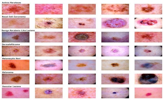
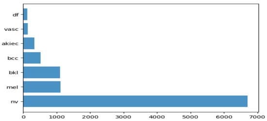
To carry out the research work, we used HAM10000 dataset (human against the machine) [39], which has 10015 dermatoscopic images and seven different classes, such as actinic keratosis (akiec) (327), basal cell carcinoma (bcc) (541), benign keratosis (bkl) (1099), dermatofibroma (df) (155), melanocytic nevi (nv) (6705), melanoma (mel) (1113), and vascular skin lesions (vasc) (142). Seven types of lesions [29] are shown in Figure 1, along with their occurrences in Figure 2, where the x-axis represents the type of lesion and the y-axis represents the corresponding count. The same dataset was divided into training, testing, and validation sets so that there was no discrepancy in the results.

Figure 1. Seven different types of diseases are caused by lesions.

Figure 2. Occurrence of images of each type of skin cancer.

2.2. Transfer Learning Nets

In this section, the focus is on transfer learning and the models used in the research are discussed briefly [40]. Transfer learning is a machine learning method in which a model developed from one task is reused in another. It is generally used when we do not have enough training data. However, the data issue can be solved with data augmentation. The main reason why we need transfer learning is that Melanoma and benign lesions have high similarities, so it takes a long time to identify and classify them. Furthermore, transfer learning is more efficient in classifying between similar lesions, making it a first choice. Transfer learning nets are trained on large datasets and their model weights are frozen, and the last few layers are changed for a different dataset. In this paper, the models we used for comparison were VGG19, InceptionV3, InceptionResNetV2, Resnet50, Xception. and MobileNet. However, here, we not only used the frozen weights, but we also retrained them on our dataset so that the network layers had better precision in distinguishing between seven different types of lesions. We trained the models on the skin lesion dataset using these six transfer learning nets and analyzed their predictions. In addition to this, we plotted their training and validation loss, training and validation accuracy, along with their individual confusion matrices. A comparative analysis of accuracy of all these learning nets was then performed, and we determined the net that gave the highest accuracy in identifying all the lesions.

2.2.1. VGG19

This network is characterized by its simplicity. It has five blocks each of 3 × 3 convolutional layers stacked on top of each other. Volume size is reduced by max-pooling of 2 × 2 kernels and a stride of 2. It is followed by two fully-connected layers, each of 4096 nodes, with a ReLU activation function. The final layer has 1000 nodes with softmax as its activation function [41]. VGG19 has about 143 million parameters in total. Some applications of the VGG net are mentioned by Canziani [31] in his paper.

2.2.2. InceptionV3

InceptionV3 [42] is the refined version of the GoogLeNet architecture [43]. The basic idea of this net is to make this process simpler and more efficient. The Inception module acts as a multi-level feature extractor. It computes 1 × 1, 3 × 3, and 5 × 5 convolutions within the same module of the network. The outputs of these filters are then stacked on each other and fed into the next layer in the network.

2.2.3. InceptionResnetv2

In this net [44], the residual version of Inception nets is used rather than simple inception modules. Each Inception block is followed by a filter-expansion layer (1 × 1 convolution without activation), which is used for scaling up the dimensionality of the filter bank before the addition to match the depth of the input. Inception-ResNet-v2 matches the computational cost of the Inception-v4 network. The difference between residual and non-residual Inception variants is that in the case of Inception-ResNetv2; batch normalization is used only on top of the traditional layers, but not on top of the summations.

2.2.4. ResNet50

These are the deeper convolutional neural nets, which make use of skip connections [45]. These residual blocks greatly resolve gradient degradation and also reduce total parameters. Residual Networks (ResNet [46]) architecture follows two simple design rules. Firstly, for the same output map size, layers have the same number of filters, and secondly, when the feature map size is halved, the filters count is doubled. Batch normalization is performed after each convolution layer and before the ReLU activation function. If the input and output have the same size, the shortcut is used. When there is an increase in dimensions, the projection shortcut is used.

2.2.5. Xception

The Xception [47] architecture is an extension of the Inception architecture. It replaces the standard Inception modules with depth-wise separable convolutions. It does not perform partitioning on input data and maps the spatial correlations for each output channel separately. The Xception net then performs 1 × 1 depth-wise convolution, which captures cross-channel correlation. It slightly outperforms Inception V3 in terms of smaller data and vastly on bigger data.

2.2.6. MobileNet

This net makes use of depth-wise separable connections, similar to the Xception net. For MobileNets [48], the depth-wise convolution applies a single filter to each input channel. The pointwise convolution then applies a 1 × 1 convolution to combine the outputs of the depth-wise convolution. A standard convolution layer does both: filters and combines inputs into a new set of outputs in one step. The depth-wise separable convolution splits this into two layers: a separate layer for filtering and a separate layer for combining. This factorization has the effect of drastically reducing computation and model size. MobileNet is particularly useful for mobile and embedded vision applications. It has fewer parameters compared to others and also less complexity. This architecture is a concise form of the Xception and Inception nets.

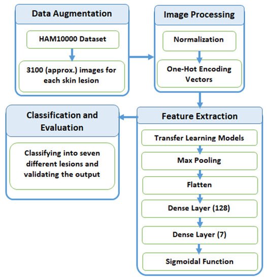
2.3. Proposed Methodology

In this section, we explain the process of classification of skin lesions. The main issue with the dataset is that it is highly imbalanced and contains a lot of duplicated images. Therefore, we made use of data augmentation to resolve this issue. Figure 3 provides a diagrammatic representation of the proposed method.

Figure 3. Process flow diagram of the proposed method.

2.3.1. Data Augmentation

When inspecting the dataset, it was observed that a lot of images were just a replication of each other, which is not beneficial for our models. We identified the unique images in the dataset, which amounted to be around 5514. We split these images into training and testing data of 80% and 20%, respectively. Training data were further divided into 90% training and 10% validation. Training data had approximately 4000 images, which was very few, and also, the classes were unbalanced because a few classes had many more images compared to others. After removing duplicates, Melanocytic Nevi had 3179 images and Dermatofibroma had only 28 images. We tackled this problem by replicating the class with low data by multiplying it by a factor that would produce data close to the class with the highest data.

Table 1 explains the frequency of images of each label before and after augmentation. All the images were multiplied by a factor k so that they could lie closest to Melanocytic Nevi. The above technique was used to avoid the problem of class imbalance. Here, we expanded the training dataset artificially. We altered the training data with small transformations to reproduce variations. A few techniques, such as rotation, zooming, and shifting vertically and horizontally, were implemented. All the images were part of the HAM10000 dataset, and their dimensions were resized from 450 × 600 to 128 × 128 dimensions for convenience in processing.

Table 1. Data augmentation of the dataset.

Disease	Frequency before Augmentation	Multiply Factor (k)	Frequency after Augmentation
Melanocytic Nevi	3179	1	3179
Benign Keratosis	317	10	3170
Melanoma	165	19	3135
Basal Cell Carcinoma	126	25	3150
Actinic Keratosis	109	29	3161
Vascular Skin Lesions	46	69	3174
Dermatofibroma	28	110	3080

After training the model with the initial training dataset, it was observed that even though a good accuracy was obtained, an observation of the classification matrix reflected the real picture. One class (Melanocytic Nevi) was classified a majority of the time since it had the highest frequency. This indicated that the model was biased and was not able to predict or classify other low-frequency classes. To overcome this situation, it was required to equalize the distribution of classes and let the model understand each class. The dataset was augmented by increasing the frequency of each class so that all the classes had the same number of images. As a result, a better performing wholesome model could be realized.

2.3.2. Preprocessing

After the image acquisition task, we performed image preprocessing. We had three channels of data corresponding to the colors Red, Green, and Blue (RGB). Pixel levels are usually [0–255]. Image preprocessing involves the normalization of the images. In normalization, the mean and standard deviation of all images in the dataset is calculated. The mean of all the images was subtracted from the initial images and then the obtained result was divided by standard deviation. On the other hand, the seven diseases were one, hot encoded, i.e., a binary column for each category was created.

Image width, image height = 128, 128

3, channels = pixel levels in the range [0–255]

where x is the original feature vector, μ is the mean, and σ is the standard deviation.

2.3.3. Feature Extraction

Feature extraction is the most crucial step in classification. Feature extraction was carried out by pre-trained transfer learning models. This involves looking up important features in an image and then deriving information from them. Several CNNs are stacked up back-to-back in order to make a model.

Here, we used pre-trained models, such as VGG19, InceptionV3, Resnet50, Xception, InceptionResNetV2, and MobileNet. All of the above pre-trained nets used the weights of the Imagenet. The bottom layers were Max Pooling, which calculates the maximum value of each patch of the feature map, Flatten, which converts the 3d array into a 1d array, Dense layer with 128 neutrons, and finally, a Dense layer with seven neurons, corresponding to seven different diseases with a sigmoidal activation function.

2.3.4. Classification and Evaluation

The final layer outputs an array of seven values, which indicates the probability of each category of disease. The class number was in correspondence to seven different skin cancers. The class numbers assigned for different lesions were actinic keratosis (0), basal cell carcinoma (1), benign keratosis like lesions (2), dermatofibroma (3), melanocytic nevi (4), melanoma (5), and vascular skin lesions (6), and in the evaluation phase, we used a validation dataset for validating the different nets for the skin lesion dataset.