Your browser does not fully support modern features. Please upgrade for a smoother experience.
Please note this is an old version of this entry, which may differ significantly from the current revision.
Subjects:
Engineering, Environmental
In the design of the monitoring system, microclimate monitoring system was decided that it should consist of ultra-low power autonomous wireless sensors using transmission techniques capable of coping with the particularities of historic buildings and, at the same time, that the batteries should last for years without the need for maintenance.
- wireless microclimate monitoring system
- wireless sensor node
- thermic sensors
1. Description of the Microclimate Monitoring System
In the design of the monitoring system, it was decided that it should consist of ultra-low power autonomous wireless sensors using transmission techniques capable of coping with the particularities of historic buildings and, at the same time, that the batteries should last for years without the need for maintenance. For data collection, a gateway should be developed capable of receiving sensor transmissions, aggregating them, pre-processing them, and transmitting them to the cloud via an Internet connection. Finally, an infrastructure should be provided to store and process environmental data in real time, which should always be available and accessible by the user. Thus, it was decided that the best option was to deploy a cloud computing system accessible to users through the Internet via a web browser. This approach is in line with the concept of the Internet of Things (IoT) and is rapidly being incorporated into smart building solutions [52].
As a result of these requirements, a system was designed and deployed, the diagram of which is shown in Figure 1. It is comprised of ultra-low power wireless sensor nodes, a sink gateway in charge of collecting data transmissions, and cloud infrastructure.
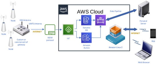
Figure 1. Diagram of the wireless microclimate monitoring system.
The wireless sensor nodes, depicted in Figure 2a, are built around an ultra-low power C8051F920 microcontroller (Silicon Laboratories Inc., San José, CA, USA), a SHT15 temperature and humidity sensor (Sensirion, Staefa ZH, Switzerland) with a typical accuracy of 0.3 °C, a CC1101 radio modem (Texas Instruments, DA, USA), and a high-density 3.6 V, 1 Ah Lithium-thionyl battery. Data are transferred wirelessly to the gateway using the 868 MHz European unlicensed industrial, scientific, medical (ISM) band, Gaussian frequency-shift keying (GFSK) for the modulation, and a fixed transmission frequency for all the sensor nodes. This sensor node is an adaptation of a previous one devoted to the detection of xylophagous [53] that copes adequately with the requirements of lifespan and long distances and tick walls of historical buildings.
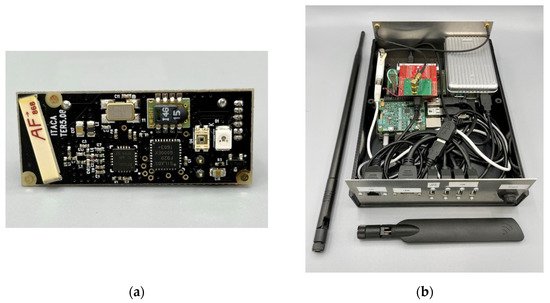
Figure 2. Key components of the electronics associated to the monitoring system: (a) wireless sensor node with a size of 4 cm × 1.5 cm × 1.5 cm, (b) custom gateway designed specifically for the monitoring needs in cultural heritage sites.
The gateway, shown in Figure 2b, was built to be as flexible as possible in order to experiment with different approaches, so it was decided to implement it around a Raspberry Pi 3 board (Broadcom Inc., San Jose, CA, USA) and the Linux operating systems. Suitable hardware was added to this base system in order to support the functionality: a CC1101 radio module and an STM32L04 microcontroller (STMicroelectronics N.V., Geneva, Switzerland) to receive the transmissions of the sensor nodes, and a 3G USB dongle to provide mobile connectivity to Internet, and, considering that the gateway is connected to the mains power, a rechargeable lithium-ion battery to provide energy to the gateway during power outages. The main task of the gateway is to collect wireless transmissions of the sensor nodes, store them temporarily in a local database, and transmit them to Internet when connectivity is available. The data transfer is implemented using the MQTT [54] client server publish/subscribe messaging transport protocol.
For the implementation of the cloud infrastructure, it was decided to choose the offering from Amazon Web Services (AWS). The MQTT messages are processed by the AWS IoT cloud service in order to split the message in sensed magnitudes such as temperature, humidity, or light level (humidity and light not used in this work), as well as in communication-related parameters (e.g., received signal strength indicator, battery level, and message counter). These two types of data flows are stored in a NoSQL AWS DynamoDB database and in an SQL AWS AuroraDB, respectively. In order to allow data access through web browsers, a Linux virtual machine was deployed in the AWS EC2 service which runs a Redash [55] data visualization dashboard. For statistical analysis, all data collected along the monitored period could be downloaded locally using AWS Data Pipeline service. For the ambient sampling strategy of the monitoring system, the time between two consecutive measurements (and transmissions) was set as a random variable following an exponential statistical distribution with a mean of one hour; the initial purpose of this transmission pattern was to decrease the probability of data transmission collisions and to provide statistically independent sample points. As described below, this strategy became problematic for the data treatment, so it has been discarded in subsequent designs, following fixed sampling patterns based on standards such as UNI 10829:1999 [56], EN 15757:2010 [7] and ASHRAE 2011 [57]. As a reference, [58] reviews the standards and procedures suitable for creating a monitoring system dedicated to cultural heritage. In that work, a wired solution with 3G connectivity is proposed to cover specific needs that this particular IoT solution cannot cover, e.g., sampling rate, and equipment redundancy.
2. Sensor Calibration
When a set of thermic sensors is implemented for monitoring a confined environment, small differences are expected among the sensors. As undertaken by other authors [59,60], a bias correction was performed prior to their installation by considering the mean value of all sensors as the true temperature according to a calibration experiment carried out. Firstly, 26 sensor nodes were placed together inside a climate chamber of 23 m3 driven by a ceiling air cooler (Küba Comfort DP model DPB034) at a controlled temperature, increasing from 26 up to 30 °C for three hours. Next, the temperature inside the chamber was reduced to 16 °C for less than one hour. This calibration experiment lasted for 320 min, and the number of measurements recorded by each sensor fluctuated between 491 and 550, which implies one value collected every 35–41 s.
Once the experiment finished, the mean temperature recorded by each sensor was computed for both the hot and cold stages. Next, the correlation between both parameters was checked in order to discuss if the bias resulting from the calibration at the cool stage was similar to that obtained at the hot stage. This bias was calculated for each sensor by subtracting the mean temperature recorded by that node with respect to the grand mean collected by all nodes together. Finally, all temperatures collected during the microclimate monitoring experiment by a given node were corrected by subtracting the corresponding bias.
For each node, the mean temperature (Tmean) during the calibration in the hot stage was computed by averaging the first 320 values. Next, the minimum temperature was obtained for the cool stage. It turned out that both parameters are positively correlated (r = 0.743, p < 0.0001), which suggests that trajectories from both calibration stages are approximately parallel for the set of sensors. In the hot stage, the node marked as UP4 (node labels described in the next section) was the node with highest mean (Tmean = 28.09 °C), while the lowest mean corresponded to EN1, Tmean = 27.48 °C. Figure 3 shows the time series of temperature in the calibration experiment for both nodes. Their trajectories are parallel during the whole experiment, which implies that the sensor bias can be assumed as equal for the hot and cool stages (i.e., the bias does not depend on temperature).
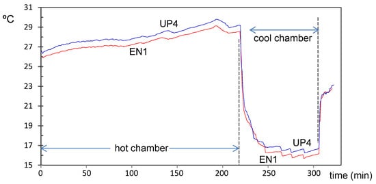
Figure 3. Trajectories of temperature during the calibration experiment, corresponding to nodes EN1 (in red) and UP4 (in blue). A parallel pattern is observed both for the hot and cool stages.
The difference between Tmean of UP4 and EN1 is 0.61 °C, which is consistent with the accuracy of the Sensirion SHT15 (±0.3 °C) in the range of temperatures used for the calibration. In this design, it was decided to select the most accurate model of the SHT1x series, in contrast to previous projects [53] where Sensirion SHT10 was utilized to optimize the cost of the solution. Currently, Sensirion SHT1x series are currently deprecated, based on our experience we would recommend using Sensirion SHT3x series sensors for the new designs.
By comparing Tmean values of each node, derived from the calibration experiment, it was found that the Tmean of RE4 was the one closer to the grand mean calculated using all nodes. Hence, a null bias was considered for RE4.
As the calibration experiment at the hot stage lasted longer than the one at the cool stage, the estimated bias is more accurate. Thus, it was decided to compute the bias of each sensor by subtracting the mean temperature recorded during the hot stage (Thot) minus the Thot of the reference node RE4. It was checked that the resulting temperature biases (Table 1) follow, approximately, a normal distribution with mean equal to zero and standard deviation s = 0.16. Given that the present research intends to discuss small differences of temperature, it is necessary to achieve the maximum accuracy in all measurements. Thus, the original values were corrected with the bias corresponding to each node, by subtracting every recorded value minus the bias indicated in Table 1.
Table 1. Temperature bias (°C) for each node, derived from the calibration experiment.
| Node | Bias | Node | Bias | Node | Bias | Node | Bias |
|---|---|---|---|---|---|---|---|
| CH1 | −0.075 | LO1 | −0.003 | RE1 | −0.036 | UP1 | −0.277 |
| CH2 | 0.012 | LO2 | 0.069 | RE2 | −0.046 | UP2 | −0.098 |
| CH3 | 0.083 | LO3 | −0.088 | RE3 | −0.249 | UP3 | 0.276 |
| EN1 | −0.280 | LO4 | 0.077 | RE4 | 0.000 | UP4 | 0.335 |
| EN2 | 0.097 | LO5 | 0.009 | RE5 | 0.150 | UP5 | 0.175 |
| EN3 | 0.160 | LO6 | −0.019 | RE6 | 0.189 | ||
| OUT | −0.028 | LO7 | −0.089 | SAC | −0.115 |
The calibration procedure used in this work might be arguable because a reference sensor calibrated by the manufacturer should be required for an accurate estimation of the real bias [61]. Nevertheless, the present work intends to characterize the relative differences of temperature inside the building, and hence knowing the exact real bias of each sensor is of no interest in this case. Other authors [59,60] have found that this approach is adequate for making comparisons between sensors.
In [58], different thermal insulation materials were tested, and a reliable calibration was needed for this purpose. To achieve this goal, it is necessary to know the true value of temperature with precision. So, precalibrated industrial sensors with high accuracy were selected. In the present work, this is not necessary because PCA deals with differences and not with the true values.
3. Installation of Wireless Sensor Nodes
A total of 26 sensors were installed in the church. This number is a balance between budget availability and the size of the building to be monitored. Another work [58] used an infrared thermography method for deciding the best position of sensors. This method helps to map the superficial thermal conditions of the walls; therefore, it is a qualitative way to verify the absence of thermal anomalies in the original wall. In the present work, this approach is not suitable because we are studying air temperature differences.
As indicated in the description of the monitoring system, the aim was also to make the deployment as quick and simple as possible in order to minimize interference with the tempo services and, of course, without affecting the state of conservation of artworks and buildings. In this sense, the set-up of the gateway consisted of simply powering it on, and the installation of the sensors consisted of dropping them at the point of interest manually or by means of a pole (Figure 4a). However, for those located at higher elevations, specialized personnel were required to clamp them to the security banister of the cornice on top of all pilaster capitals around the entire perimeter of the central nave (Figure 4b). One morning was spent on the installation of the lower nodes and another morning deploying the upper nodes.
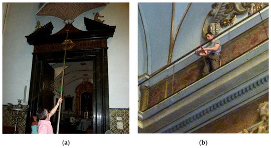
Figure 4. (a) Installation of sensor nodes at heights up to 9 m. (b) Installation of the sensor nodes clamped at above 12 m to the security banister of the cornice on top of all pilaster capitals around the entire perimeter of the central nave.
Several criteria were considered to decide the position of nodes given the quantity of available nodes. Figure 5 shows positions and heights of the sensor nodes. For example, six of them, coded as UP1 to UP4 and R5, R6, were located at heights higher than 12.1 m in order to assess the upper environment close to the ceiling vaults; three nodes were placed at the Communion Chapel (CH); six at the retable decorating the presbytery (RE); seven were spread out at different low points (LO) of the central nave (at a height between 2 and 3 m); and three were conveniently positioned to evaluate the indoor air conditions near the main entrance (EN). Another node was located at the corridor leading to the sacristy (SAC) and the last one was positioned outside the church (OUT). Considering that the outer doors of the temple are open at least six hours per day, an additional node was installed inside the narthex (EN) in order to assess the environment here, which can be regarded as intermediate between air conditions at the central nave and outside the building. Apart from the Communion Chapel, narthex, and the corridor, which can be considered as somewhat independent chambers, the target was to characterize the indoor temperature according to height and distance from the principal entry, which is the main source of airflow exchange. Trying to prevent nodes from being manipulated unintentionally, they were properly positioned to minimize their visibility and to not be easily reached by people. For this reason, none of them were put very close to the floor level.
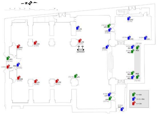
Figure 5. Position of the 26 nodes installed at the church of Saint Thomas and Saint Philip Neri (Valencia). Color codes according to their height (h): red (h < 3 m), blue (3 < h < 6 m), green (h > 6 m). The position of the sink gateway is indicated as SG. The retable is depicted in grey.
Table 2 indicates the height of each node. Those located at the Communion Chapel, coded as CH (chapel), are the following:
Table 2. Distance of the nodes (height, in m) from the floor level of the central nave of the church.
| Node | Height | Node | Height |
|---|---|---|---|
| CH1 | 4.2 | RE1, RE2 | 4.0 |
| CH2, CH3 | 3.7 | RE3, RE4 | 8.6 |
| UP1, UP2, UP3, UP4 | 12.1 | RE5, RE6 | 12.2 |
| UP5 | 5.0 | EN1, EN2 | 2.5 |
| LO1, LO2, LO3, LO6 | 2.0 | EN3 | 4.3 |
| LO4 | 3.9 | SAC | 3.5 |
| LO5, LO7 | 5.0 | OUT | 2.0 |
This entry is adapted from the peer-reviewed paper 10.3390/s21237795
This entry is offline, you can click here to edit this entry!