Silicon micro-strip detectors are fundamental tools for the high energy physics. Each detector is formed by a large set of parallel narrow strips of special surface treatments (diode junctions) on a slab of very high quality silicon crystals. Their development and use required a large amount of work and research. A very synthetic view is given of these important components and of their applications. Some details are devoted to the basic subject of the track reconstruction in silicon strip trackers. Recent demonstrations substantially modified the usual understanding of this argument.
- silicon micro-strips
- tracker detectors
- positioning algorithms
- least-squares method
- track reconstructions
1. Properties and Operation of Silicon Micro-Strip Detectors
The study of matter at extreme conditions requires collisions of elementary particles at the maximum energies allowed by the actual accelerators. Detailed analysis of the reaction products of those collisions enable the extraction of the physical parameters relevant for this study. The reaction products are a large set of other particles, some stable or of sufficiently long half-life to cross the nearby detectors. Charged particles are easily detected for their streams of ionization released in solid or gaseous matter. The neutral components of the reaction products require other very special detectors, able to transform their energy in detectable signals. The stream of ionization of the charged particles in solid or gaseous materials is a fundamental source of information about the properties of the incident particles, therefore, large efforts are dedicated to the observation and measurement of their ionization streams. Evidently, the amount of ionization, on the unit of path length, is an essential parameter for the quality of the detectors. The average ionization released in a solid silicon slab is around ten times that released in a gaseous detector. The production of an electron-hole pair, in a silicon detector, requires an average of 3.6 eV. Instead, the average ionization is around 30 eV in a gaseous detector. However, the collection of the charges released in silicon slabs is a much more elaborate operation than the equivalent operation in gaseous detectors. Thus, only in recent years, silicon detectors acquired extensive applications. The huge use of silicon crystals, in all the electronic devices, drastically reduced the high production costs of silicon crystals of the best quality (detector grade) required by the detector construction. Further details and plots on this subject can be found in Refs.[1,2].
For its electronic composition, a silicon crystal is a semiconductor, having a resistivity of 400 kW cm at 300 K, intermediate between that of a conductor and that of an insulator. Impurities and crystal imperfections give an effective resistivity around 10 kW cm [2], for mass production crystals. The effects of this reduction in resistivity, of the higher quality crystals, can be compensated resorting to the properties of reverse-biased diodes. In fact, in a semiconductor, the density and the type of current carriers can be tuned with the addition of appropriate impurities, able to add electrons to the conduction band or holes to the valence band, giving n-type or p-type material. The surface treatments of an n-type or p-type materials with the impurity of opposite property produce the diodestructures (diode-junctions). The geometrical dispositions of those impurities on a surface can transform a slab 300 µm thick (the typical thickness of a detector) in an array of parallel lines of diode-junctions: a micro-strip silicon detector. The anisotropy of the impurity distributions has a drastic effect on the current conduction, allowing only the conduction for a given sign of the applied tension. Applying a reverse-bias (i.e., the tension that can not conduct the current in the diode), the density of the charge carriers is reduced in the thickness of the slab. The depletion from free charge carriers, of the detector active region, eliminates the recombination with the charges released by the ionizing particle, keeping intact the incoming ionization distribution.
The reverse-bias is increased to obtain the largest allowed depleted region. The reverse-bias has a maximum beyond which the electric field can accelerate the charge carriers (always present, even if in negligible concentrations) above the ionization of the material, generating a rapid rise of the diode current. Therefore, to have a detection, the maximum bias can not be reached. As an ionizing particle crosses the depleted region, the applied bias guides the two types of produced charges toward the corresponding collecting electrodes. In the actual experiments, the energies of the charge particles move their ionization release in regions with a relative minimum. Charged particles of this type are indicated as minimum ionizing particles (MIPs). Evidently, the particle detectors must efficiently operate for the MIPs. The charge released is proportional to the thickness of the depleted region. However, this region, and the thickness of the detector, must be limited to avoid that the hard scattering of the MIP, with the constituents of the crystal (multiple Coulomb scattering), randomly deviates the particle from its path. For a MIP in a silicon detector, 300 µm thick, the most probable number of electron-hole pairs is ≈ 23,000, collected by the corresponding electrodes in a few tens of nanoseconds. To handle such low charges, consistent amplifications with very low noise amplifiers are required. Hence, the strips of diode junctions are connected to the charge amplifiers thought decoupling capacitors (AC connection). These capacitors are easily produced with a thin layer of silicon oxide. The array of charge preamplifiers are realized in very large integration device (custom produced) with a separation, of the component amplifiers, equal to that of the strips; they are optimized for the corresponding applications [2] (Refs. [3,4] for those used in the CMS and ALICE trackers). The preamplifiers and their service electronics are contained in a different component (often called "hybrid"). Each preamplifier, of the array, is wire-bounded to the corresponding strip. A schematic set-up of a silicon micro-strip detector is represented in Figure 1 on the junction side.
Double sided strip detector. The structure of the micro-strip detectors discussed above, contains only a parallel array of linear diodes, evidently this structure allows the measurement of a single coordinate of the path of a MIP relative to the silicon surface (another coordinate is always given by the position of the sensor plane in the supporting mechanical structure). To measure the other coordinate, an additional detecting layer is required, with its strips orthogonal to the previous one. The combination of the two detections increases the random disturbance of the multiple Coulomb scattering to the particle tracks and augments the complexity of the trackers, and the weight for the satellite experiments [5] (Figure 2, array of double sided micro strips for a the PAMELA satellite). To eliminate a second detector, the other surface of the silicon slab, opposed to that with the array of diode-junctions, is armed with a set collecting electrodes oriented orthogonal to the direction of diode junctions [5–7]. Various specialized implants are required for the proper functioning of this second detecting layer (conventionally called ohmic side, Figure 1), among them, this side must be instrumented with preamplifiers and service electronics whose reference is not the ground, as usual, but the depleting bias. Special types of power supplies are required to distribute the electric currents necessary for the operation of the preamplifiers and the service electronics 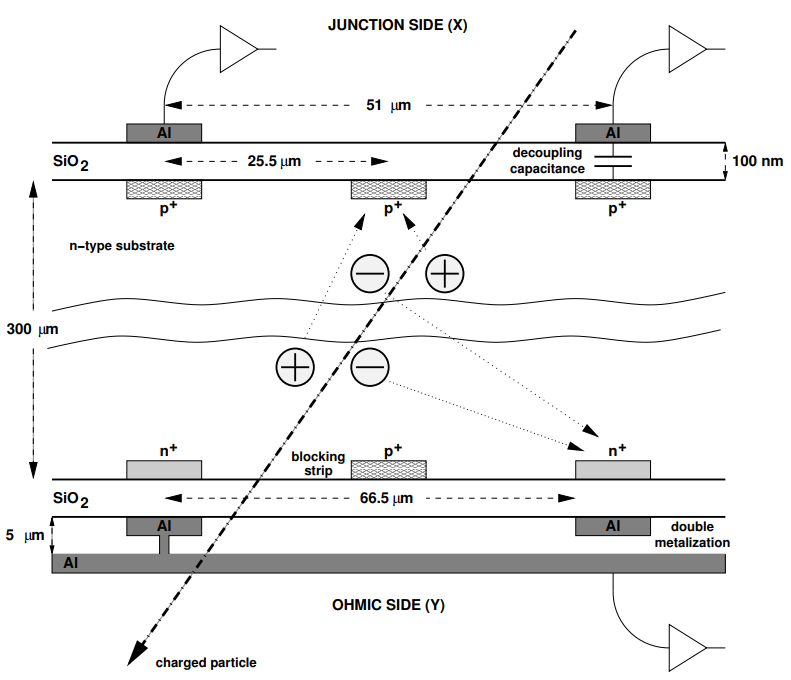 Figure 1. Schematic set-up of a double-sided micro-strip detector, the junction side is the set-up typical of the single side micro-strip detector.
 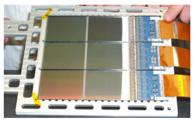 Figure 2. Array of double sided micro-strip detectors for the payload for antimatter matter exploration and light-nuclei astrophysics (PAMELA) satellite experiment. The right side of the detector
layers shows the connections to the service electronics.
3D micro strips. Recent developments of silicon detectors explore the possibility to confine the diode structure in deep holes orthogonal to the layer surface. As usual, a depleting bias is provided and now the electric field collects the released charges toward the nearest hole. The signals from an array of holes are collected by an external electrode (strip). The 3D micro-strips [8] are conceived to better sustain the huge radiation damage of the high luminosity large hadron collider (LHC).
Forms of the charge distributions. The charges of each sign, released by the ionizing particles drift toward the collecting electrodes with a constant velocity (different for the electrons and the holes) proportional to the local electric field. During their drifting times the electron and the holes are subject to a diffusion due to the thermal fluctuation of the medium (further mathematical details in Ref. [9]).
Assuming a continuous charge distribution along the particle track, the forms of the charge density at the detection plane can be calculated as in Ref. [9]. The projected distributions on a plane orthogonal to the strips are reported in Figure 3. The combination of drift and diffusion contributes to the form of the charge distributions arriving to the collecting electrodes. The sole drift in the electric field gives rectangular distributions with a side equal to the projection of the track on a direction orthogonal to the strips.
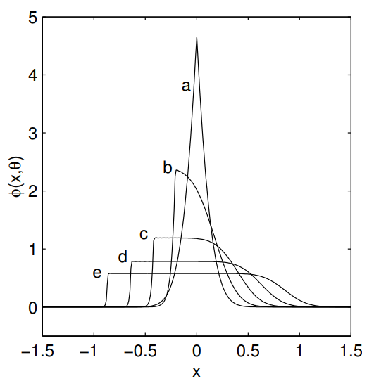
Figure 3. Forms of the charge distributions (all normalized to one) at various incidence angles calculated with a continuity assumption. The curves a, b, c, d, and e are, respectively, for θ = 0◦, θ = 5◦, θ = 10◦, θ = 15◦, and θ = 20◦ (from [9]).
The forms of Figure 3 can be considered averages over very large numbers of realistic distributions. In fact, the actual distributions are produced by a finite number of charges released along the particle track. This number fluctuates as a Landau distribution with the parameters corresponding to the crossed material. In addition, each segment of any track has itself a Landau distribution of released charges, according to the segment length. Each charge follows a random walk resulting from the combination of drifting and diffusion or scattering by the thermal fluctuations of the crossed medium. Along the track, some electrons acquire an energy well above the mean value of the other charges (d-rays) and produce the tails of the Landau distributions above their most probable values. Thus, a large set of signal fluctuations must be expected as output of the strip preamplifiers.
Strip calibrations. The reconstruction of the particle signals in the detector requires some detailed operation on each strip. The outputs of the each strip-preamplifier are converted in a number by the analog digital converter (ADC). These numerical data require corrections with some strip parameters. The pedestals and strip noise must be calculated in absence of particle signals. The pedestals and the strip noise are constants and are calculated (or recalculated) when the status of the detector is supposed to be changed. Another parameter (defined as common noise) must be determined on event by event basis, it is particularly relevant for double sided detectors. The common noise is produced by the fluctuations of the power supply and other electromagnetic interferences, and it is constant for all the preamplifiers contained in the same integrated device. An iterative procedure allows the definition of these parameters (also discarding possible particle hits). A set of random triggers is generated, the first iteration supposes the absence of the common noise and the output of each strip is averaged for all the triggers. This average eliminates the noise of the read-out electronics and defines the effective zero (pedestal) of the strip signal. With the initial set of pedestals, the common noise for each trigger is calculated as the difference of the strip output and its pedestal averaged over all the strips connected to the same integrated amplifier device. This first set of common noise is subtracted from the output of each random trigger and a new set of pedestals is generated. These iterations are repeated until convergence. The strip noise is given by the root mean square of the differences of the strip outputs minus the pedestal and minus the common noise. The large majority of the strips have very similar noises, a small fraction (usually less than 5%) have higher noise. The noisy strips require a special attention in handling their data.
Cluster detection. The signals released by the charged particles (the MIP in particular) require careful criteria to distinguish them from the background noise. The forms of Figure 3 suggest that the particle signal distribution is spread on a small group of nearby strips: a cluster. To reduce the probability of false detections, a strip is inserted in a cluster if its signal is at least few times the strip noise. This threshold is tuned on the characteristic of the tracker detector and to efficiency required for the detection. Some experiments defines the seed of the cluster to be up to 7 times the corresponding strip noise. The other component of cluster are selected with a lower threshold. If several adjacent strips are classified as seed, the strip with the highest signal-to-noise ratio is the cluster seed. Additionally, the global quality of the cluster can be tested exploring its global signal-tonoise ratio. The cluster detection requires a due care to the inclusion (or exclusion) of the noisy strips.
Hit positioning. Typically, silicon micro-strip detectors are composed in regular arrays (called trackers) in a mechanical support structure finalized to reconstruct the paths of the incoming charged particles. The addition of a magnetic field allows the extraction of the particle momentum and sign of its charge. Thus, a dedicated algorithm must be applied on the detected clusters to extract the position where the particle hits the micro-strip detector. Evidently, for its geometry, a micro-strip detector can only give a single coordinate of the track path, that orthogonal to the strip direction (another coordinate is fixed by the mechanical structure of the sensor plane and is given by other measuring systems). Even if the dimensions of the clusters are in the range of few hundred microns, at most, much more precise positions can be extracted. The quality of the hit position has a fundamental effect on the track reconstruction and on the extraction of the track parameters. The center-ofgravity (COG) of the cluster is the most used positioning algorithms. The COG (sometimes called barycenter or weighted average) is defined by Xg = (∑i CiYi)/(∑ Ci), where Ci is the charge released in the strip i whose center (orthogonal to the strip direction) is in Yi. This definition must be used with the due care. In fact, as discussed in Refs. [9,10], a set of systematic errors and anomalies are contained in this very simple definition. The first set of anomalies are gaps in the COG distributions that depends from the size of the charge distribution and the number of strips inserted in the COG algorithm. In general, an even number of strips generates gaps around Xg = 0, instead, an odd number has gaps around Xg = ±1/2 (the strip length is put to be one). As consequence, the corresponding probability density functions (PDFs) of positioning errors turn out to be very different. The PDFs, calculated in Refs. [11,12] illustrates these differences. To limit the influence of different PDFs, the same number of strips should be inserted in the COG calculation. This implies to neglect part of the information contained in the cluster, for clusters larger than the average, or insert strip-signals discarded by the algorithm of the cluster construction. Each case has a negligible effect on the hit position reconstruction. In fact, large clusters are produced by the high side of the Landau PDF and each of its strips has a good signal-tonoise ratio, thus the elimination of a lateral strip has a small effect on the result. Similarly, for the clusters with a lower number of strips, they are given by the low charge side of the Landau PDF, with a low signal-to-noise ratio, the addition of another strip add a small part of signal. In any case, the hit quality is low and the addition of another strip-signal has a negligible effect on the hit resolution. This recipe is useful for clusters formed by a single strip where the COG algorithm can not be used.
Another very important weakness of the COG algorithm is a systematic error contained in its position determination [9,10]. An effective algorithm (called h-algorithm) was defined in Ref. [13], further refinements are contained in Refs. [9,14], converging toward the elimination of this error. With h-correction, the hit positioning has only a random noise, becoming an unbiased position estimator. Its variance can be further reduced by a best fit with other hits of the particle in the detecting layers of the tracker.
Track fitting. The final use of the silicon micro-strips is in the track reconstruction in tracker detectors. These detectors are always immersed in homogeneous magnetic fields that impose to the incoming particles circular paths in the direction orthogonal to the field direction (helical paths in three dimensions). The radius of each circle is proportional to the particle momentum orthogonal to the magnetic field (transverse momentum). The arrays of micro-strips are arranged to optimize the measurement of the track bending and the extraction of the transverse particle-momentum. For example, the micro-strips are arranged in cylindrical surfaces if the magnetic field is directed parallel to the beam pipe of the accelerator (as in CMS [3] or ALICE [4]). The track fitting is always done with the standard least squares (sometimes called linear regression) even if for various necessity is implemented as the Kalman filter. The key point of these fitting methods is the assumption of an identity of the variance of the measurements (homoscedasticity). Rare deviations from this assumption are allowed, the observations with variances larger than the rest of the observations are called outliers. The Kalman filter is supposed to be able to detect the rare outliers, and their elimination restores the consistency of the approach. The assumption of homoscedasticity implies an enormous simplification to the fitting algorithms. The algorithms are independent from the details of the detectors. At most, to account for substantial different technology of a given detector layer, a single parameter is introduced for all the hits of that layer.
In addition, the homoscedasticity gives equations for the extraction of the observation variance (a single value) from the mean square of the fitting residuals; equations inconsistent for real systems. Often the variance, obtained with the homoscedastic equations, is improperly indicated as an experimental determination. Another assumption is the Gaussian PDF of the hit errors. If the inconsistency of homoscedasticity is proved, the
optimality of all the fitting procedure breaks down.
Toward optimal fittings. Ref. [15,16] proved that for non-homoscedastic (heteroscedastic) systems, the use of homoscedastic algorithms implies an increase in the variance (often very large) of the estimators. Due to the definition of optimal algorithm, as that with minimum variance, each fit on heteroscedastic systems with homoscedastic fitting algorithms turns out to be non-optimal with a consistent loss of resolution. The very different analytical forms of the COG PDF of Refs. [11,12] prove that the simple neglect of the strip number differences in the calculation of the COGs introduces an evident trivial heteroscedasticity also in homoscedastic systems or increases the hit-differences in the heteroscedastic ones. Another source of heteroscedasticity is the different signal-to-noise ratio of each hit given by Landau PDF of the charge released along the track. Furthermore, the simple observation of the scatter plot of any simulation of the two (or three) strip COG in function of the impact point (as the left side of Figure 4) shows immediately the impossibility of a single variance for each COG value. It must be recalled that also the histogram of the two strip COG (or three strip) shows substantial variations. These can only be generated by large variations of the probability, for the noise, to produce a given COG value for each position on the strip width (uniform population of hits on the strip is always assumed). This correlation is sufficiently strong the be directly used in the track fitting as weight of the hit with the h positioning (the lucky model of Ref. [17]) giving a good improvement of the estimator resolutions. Better results can be obtained if effective variances, for each hit, is extracted by the two-dimensional PDFs for COG error in function of the impact points for the charge released by the MIP in the seed strip and the two lateral ones. A sample of those PDFs is reported in the right side of Figure 4. The calculated effective variances are inserted in the weighted least squares (the schematic model of Ref. [17]). Similar approximate uses of the full PDFs were suggested also by Gauss [18] in his book of 1821 to avoid the complexity of the full maximization of products of PDFs (a century later the method acquired the name of maximum likelihood). However, the mean variance of the estimators is further reduced with the search of the maximum likelihood (just the procedure not-recommended by Gauss for its complexity). The hit PDFs are extracted from surfaces similar to that of Figure 4 for constant values of the (two strip) COG and with the charge collected by three strips of the cluster (ref. [17] and therein references). Again these variances could not be theminima, other improvements of minor details could produce further reductions. However, the hit-error PDFs substantially differs from Gaussian PDFs, hence, the linear equations of the least squares no longer coincide with the likelihood maximization. The hit-error PDFs have heavy tails, similar to Agnesi–Cauchy PDFs, and the maximization of the likelihood can only be done with numerical methods.
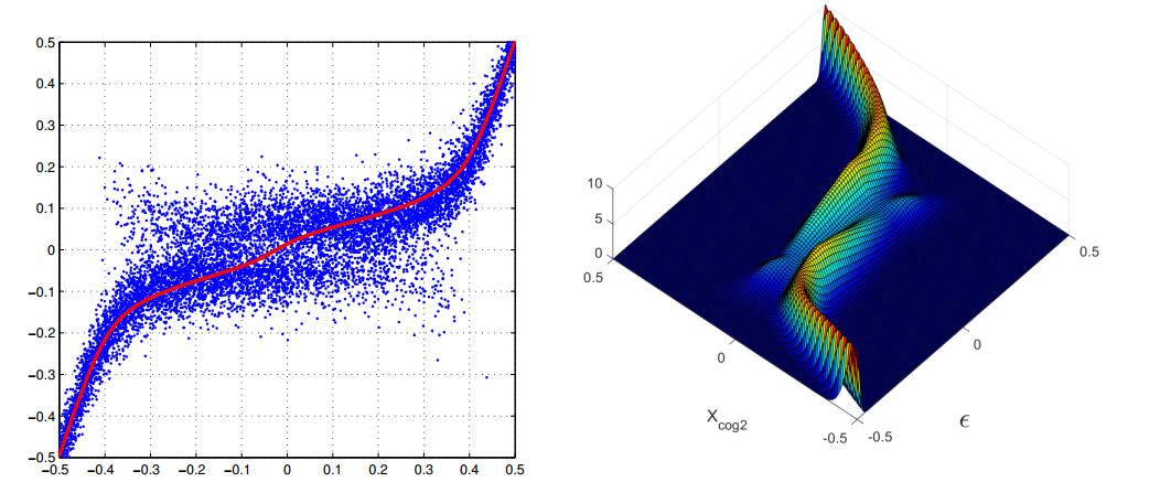
Figure 4. Left plot: Scatter plot of a two strip COG in function of the impact point for silicon strip detector of general type. Right plot: Calculated probability density function for a two strip COG (Xcog2) in function of the impact point (e) with the most probable signal released by a MIP in three strips.
2. Summary and Conclusions.
This synthetic discussion of the silicon micro-stripdetectors illustrates only essential features of these instruments. Some details are reported of their set-ups, applications and the fitting methods, specialized for high energy physics. Evidently, the use of ionizing radiations is extended well beyond high energy physics, therefore these devices find applications in a large set of industrial, medical and technological environments with dramatic increases of performance compared to the previous detection systems. However, the next upgrade of LHC, with its large increase in the reaction rates, requires additional developments of these detectors to survive to the intense radiations produced by the beam collisions and fast acquisition times to faithful reconstruct the signals released by the reaction products.
Abbreviations
The following abbreviations are used in this manuscript:
MIP: Minimum ionizing particle
COG: Center of gravity
PDF: Probability density function