Your browser does not fully support modern features. Please upgrade for a smoother experience.
Please note this is an old version of this entry, which may differ significantly from the current revision.
Subjects:
Remote Sensing
Irrigation represents one of the most impactful human interventions in the terrestrial water cycle. Knowing the distribution and extent of irrigated areas as well as the amount of water used for irrigation plays a central role in modeling irrigation water requirements and quantifying the impact of irrigation on regional climate, river discharge, and groundwater depletion. Obtaining high-quality global information about irrigation is challenging, especially in terms of quantification of the water actually used for irrigation.
- irrigation
- satellite
- soil moisture
- evapotranspiration
- water cycle
- farmers
1. Introduction
Irrigated agriculture accounts for more than 70 percent of the water withdrawn worldwide from lakes, rivers, and aquifers [1], in many countries even for more than 90 percent, thus being the greatest human disturbance in the terrestrial water cycle [2]. Even though only 17 percent of global crop land is irrigated, these lands already produce 40 percent of the world’s food [3]. Since the global demand for food will further increase in the next decades due to population growth and dietary shifts, keeping pace with this growing demand will require even further expansion and intensification of irrigated agriculture [4,5].
At the same time, urbanization pressure, market volatility, and climate variability associated with an increased recurrence and intensity of drought periods [6,7,8] have led to a call for improved water management involving reducing water withdrawals and increasing irrigation efficiency.
Meeting these ends will require: (1) modeling irrigation water requirements at the global scale [9], (2) assessing irrigated food production [10], (3) quantifying the impact of irrigation on climate [11], river discharge [12], and groundwater depletion [13,14], and (4) building plans for an optimal water resource allocation so that managers can accurately account for water use [15,16,17]. Central to all these steps is accurate knowledge about the spatial extent of irrigated lands, the amount of water applied as irrigation, and the timing when irrigation is applied.
Obtaining this information with a high quality and on a global scale, however, is not trivial. Many wells are located on private lands, are used for small-scale agriculture, and are often illegal due to the reluctance of farmers to drill wells with official permission to avoid regulations [18].
Consequently, the overwhelming majority of agricultural water use worldwide—both from groundwater and surface water—remains unmetered [19].
Earth observing satellites provide the unique ability to monitor various processes strongly related to irrigation, e.g., soil moisture, land cover, or vegetation activity, quasi-globally and frequently. In the last decade, there has been a significant interest in using satellite Earth observations to retrieve information on irrigation extent, frequency, and amount. This has led to a proliferation of studies using new satellite platforms able to measure surface variables with relatively high spatial resolutions (i.e., less than 1 km) [20]. Many studies have also attempted to include irrigation modules in land surface models or ingest satellite observations to correct for the lack of irrigation representation.
2. Irrigation Remote Sensing
2.1. Visible- and Near-Infrared-Based Methods
Visible- and near-infrared measurements can be used (i) to detect changes in vegetation greenness, health, and water content represented by empirical vegetation indices, (ii) to retrieve land surface temperature, and (iii) to model evapotranspiration. All these types of information potentially facilitate irrigation mapping and monitoring and indeed, many different strategies have been developed to do so, as will be described in the following sections.
2.1.1. Mapping Methods
Data from optical sensors including Landsat, MODIS (Moderate Resolution Imaging Spectroradiometer), AVHRR (Advanced Very High-Resolution Radiometer), MERIS (Medium, Resolution Imaging spectrometer), and SPOT (Satellite pour l’Observation de la Terre) [4,29,30,31,32], and their combination with other model-based and ground-based ancillary data [33], have been extensively used to map irrigated areas, making use of the difference in the spectral responses of irrigated and non-irrigated croplands. One of the first explicit attempts to use visible- and near-infrared remote sensing information for the detection of irrigated areas at the global scale is the International Water Management Institute Global Irrigated Area Map [23]. This dataset represented the irrigated areas of the world in 1999 with a resolution of 10 km and 28 classes. The algorithm was applied to more than 20 years of resampled AVHRR monthly time series of reflectance, combined with one year of monthly Normalized Difference Vegetation Index (NDVI) from Spot Vegetation, mean annual rainfall, a forest cover map, and a Digital Elevation Model (DEM).
Since then, there have been many other notable attempts to provide information on irrigation from the regional to the continental/global scale. For instance, Ozdogan and Gutman [32] used a supervised classification to map the irrigated area in 2001 over the contiguous United States by using a combination of Landsat and MODIS data. Ambika et al. [34] developed yearly maps (2000–2015) of irrigated areas in India based on a thresholding of 16-day composite NDVI time series from MODIS. The decision tree between irrigated and non-irrigated areas was applied on each crop class (previously produced on the basis of IRS-P6) inside each agroecological zone. The following works of Meier et al. [35], Pervez and Brown [36], Zhu et al. [37], and Salmon et al. [38] provided some updates with respect to previous works by working on census areas rather than on crop classes. A notable example is the method applied by Peña-Arancibia et al. [31] on the Murray–Darling Basin in Australia, which used a supervised classification based on the random forest technique and data not only from vegetation (in this case, MODIS NDVI), but also from hydrometeorological data, such as monthly evapotranspiration (which was simply estimated by scaling Priestley–Taylor potential evapotranspiration, ETp, via a crop factor that was derived from other satellite observations) and monthly precipitation.
Later studies focused even more strongly on the synergistic use of machine learning methods and high-resolution remote sensing data. For instance, high spatio-temporal resolution NDVI data (30 × 30 m) from the Chinese HJ-1A/B (HuanJing, HJ) satellite were used by Jin et al. [39] to separate irrigated from rainfed areas in the semi-arid province of Shanxi in China, through a novel classification method based on a Support Vector Machine (SVM). They found that not only spatial but also temporal resolution may influence the classification results. A study by Chen et al. [40] also focused on a more extended irrigation detection which includes extracting frequency and timing information through data fusion of MODIS time series, Landsat OLI data, and ancillary data. The obtained fused Greenness Index (GI) estimates with an improved spatial resolution of 30 m were found to be effective in increasing the accuracy of irrigation mapping in the Gansu Province (China). Similarly, Ferrant et al. [41,42,43] have used a random forest classifier combining Sentinel-1 (S1) and Sentinel-2 (S2) data over southern India to investigate the advantages of high-spatial resolution and a multi-sensor approach. The input resolution allowed to retrieve irrigated areas for the two Indian climatic seasons at a resolution of 10 and 20 m.
Further studies highlighted both the need of sub-kilometric spatial resolutions to differentiate very fragmented irrigated areas and the need for combining multi-sensory information (in this case, radar for soil moisture and optical for vegetation) to better separate irrigated from non-irrigated land. For instance, Demarez et al. [44] applied an incremental random forest using a combination of optical (6 Landsat-8 bands each 16 days) and Synthetic Aperture Radar (SAR) data, revealing that the combined input improves the accuracy of the classification with respect to that performed with only one source. Similarly, Pageot et al. [45] used an approach that leveraged precipitation data, reaching a similar conclusion. They also revealed that the use of precipitation data improved the performance and that the aggregation of the high temporal resolution to monthly composites resulted in similar performances while reducing the calculation time.
The increasing availability of data, processing facilities, and novel classifiers also fostered data merging approaches, including modeled data from land surface and energy balance models for the detection of irrigated land. In the work of Deines et al. [29,46], the authors used a large number of variables derived from Landsat (9 in the first version, 11 in the second version) and more than 10 covariables, such as precipitation and slope, in a supervised classifier (CART and random forest) for classifying irrigated and non-irrigated areas. The different datasets were processed in the Google Earth Engine (GEE) computing platform, producing a classification at 30 m resolution claiming an overall accuracy above 95% of detected irrigation areas. Xu et al. [47] applied a similar approach in the subhumid temperate state of Michigan.
Besides machine learning, also more simple and “conceptual” approaches were developed based on the use of a mix of land surface and energy-balance model estimates and remote sensing variables. For instance, Zohaib et al. [48] looked at the biases between three modeled variables from the ERA-interim dataset (vegetation skin temperature, surface albedo, and soil moisture) and their corresponding variables derived from MODIS and ESA’s Climate Change Initiative (CCI). McAllister et al. [49] exploited the fact that irrigated crops are supposed to be well-developed and colder than non-irrigated crops, and thus applied a simple threshold on NDVI and the difference of surface temperature to air temperature to detect irrigated areas. Similarly, Pun et al. [50] supposed that irrigated areas evaporate more than non-irrigated areas. Based on the Surface Energy Balance System (SEBS) model, they computed an evaporative fraction, and applied a simple threshold on vegetation indices and the evaporative fraction to discriminate irrigated areas.
2.1.2. Quantification Methods
Besides mapping irrigated areas, optical remote sensing can also offer some solutions for estimating the irrigation water use. Some of the approaches rely on calculating a crop coefficient and/or exploiting actual evapotranspiration (ETa) estimates from remote sensing (e.g., MODIS, Landsat, S2, S3, VIIRS, and AVHRR). For example, Le Page et al. [15] calculated the irrigation in the Tensift basin in Morocco as the difference between actual evapotranspiration and precipitation. They subtracted it from the known distributed water from dams to estimate the groundwater demand in an integrated modeling of demand and supply of water. This method exploited previous works on the determination of crop coefficients [51,52,53,54,55,56,57,58,59] to estimate actual evapotranspiration [60] by relying upon remote sensing-based vegetation indices [61,62,63,64]. The crop coefficient was also used as a supplement in a parameterized water balance approach by Saadi et al. [65] in order to show growth conditions.
Water and energy balance modeling approaches have also been investigated to assess irrigation water amounts using a combination of surface energy balance models and remote sensing data [66,67,68]. For instance, van Eekelen et al. [69] employed the surface energy balance algorithm for land (SEBAL, [70,71]) for mapping total ETa, that is split into ETa induced by precipitation (in rainfed agro-ecosystems) and ETa induced by water withdrawals. Still based on ET, Hain et al. [72] compared the estimated ETa by the Noah LSM (not incorporating irrigation) with a remotely sensed ETa product retrieved using the Atmosphere-Land Exchange Inverse (ALEXI) model over Contiguous United States. The excess ETa estimated by ALEXI was attributed to the irrigation. While large-scale irrigation agriculture could be mapped by this approach, the inherent error in Noah LSM and ALEXI ETa estimates hindered the reliability of the method in certain parts of the study area. Conceptually similar was the work of Peña-Arancibia et al. [73], who used a combination of remotely sensed data and hydrological modeling outputs to estimate the volumes of water consumed in the form of evapotranspiration over irrigated lands in two sub-basins of the Murray-Darling basin (Australia). Alternatively, Olivera-Guerra et al. [74] used Landsat 7–8 Land Surface Temperature (LST) to derive a crop water stress coefficient that was injected directly into a water balance model, and then retrieved irrigation at the pixel scale before aggregating it to the plot scale. The method was tested on wheat fields in Morocco, exhibiting good performance for estimates of seasonal amounts, but lower agreement at the daily scale.
In an attempt at using only satellite-derived ET, Vogels et al. [75] compared the ET derived from the MODIS evapotranspiration product (MOD16A2) of natural and irrigated agricultural fields to calculate the excess water or recharge, which was used as an indicator for the water available for irrigation. Somewhat similar to the study of Vogels et al., and based on the research of van Eekelen et al. [69], advances have been made in developing irrigation quantification algorithms, specifically, the so-called “ETLook” algorithm [76]. Here, the similarity of natural and irrigated pixels is defined using multiple static sources, such as a land use map, a DEM, and soil type information. Maselli et al. [77] quantified irrigation amounts with the use of NDVI derived from S2 observations over a particularly complex mosaic of rainfed and irrigated crops in Central Italy, obtaining mean biases below 0.3 mm/day and 2.0 mm/week in two sites where irrigation reference data were available.
Lastly, Aragon et al. [78] investigated the capabilities of optical Leaf Area Index (LAI) derived from the novel Planet CubeSats constellation to estimate ET for irrigation quantification purposes using the Priestley–Taylor Jet Propulsion Laboratory (PT-JPL) retrieval model over a farm in an arid region of Saudi Arabia. In this case, 3 m spatial resolution ET retrievals were used to provide information on crop water use at the precision agricultural scale.
While the above-described methods that rely on optical satellite observations have yielded promising results for mapping irrigated areas, optical data are sensitive to weather conditions and cloud cover, which limits their utility in many tropical and temperate areas.
2.2. Microwave-Based Methods
Microwaves have the advantage that they are not hindered by weather conditions, and are independent of illumination. Microwaves are sensitive to the water content in the soil surface and vegetation and therefore have the potential to monitor changes in soil moisture as a result of irrigation events.
3.2.1. Mapping Methods
In recent years, microwave satellite soil moisture products have been introduced as a tool for detecting irrigated areas. One of the first studies was carried out by Kumar et al. [79], who compared the soil moisture distribution of a modeled dataset that does not incorporate irrigation information against various coarse spatial resolution satellite soil moisture products. Assuming that the satellite products do contain the irrigation signal, it can be expected that they will also exhibit wetter soil moisture conditions if irrigation is applied. The authors concluded that, even though promising results for the detection of irrigation were found in some specific areas, the spatial mismatch between model and satellite data as well as the confounding effects of topography, vegetation, frozen soils, and Radio Frequency Interference (RFI) led to substantial uncertainties in most regions. A similar approach has been used in several other studies in Spain [80], Australia and Morocco [81], and India [82]. Lawston et al. [83] further demonstrated that not only the spatial signature but also the seasonal timing of irrigation over three vastly irrigated areas in the United States could be identified using the Soil Moisture Active Passive (SMAP) enhanced 9 km product. In contrast, Fontanet et al. [84] found that disaggregated satellite soil moisture data obtained via the Disaggregation based on Physical and Theoretical Scale Change algorithm (DISPATCH) [85] is not sensitive to irrigation when it is applied locally, i.e., at spatial scales smaller than 1 km2. Nevertheless, Dari et al. [86] showed the capability of DISPATCH downscaled Soil Moisture and Ocean Salinity (SMOS) and SMAP soil moisture data in detecting and mapping irrigation at 1 km spatial resolution over heavily irrigated portions of the Ebro River basin, in Spain.
SAR data seem to provide a new opportunity for mapping and monitoring irrigation at the agricultural field scale. Indeed, radar measurements are very sensitive to the soil water content due to the sharp increase of the soil dielectric constant associated with soil wetting. El Hajj et al. [87] observed this effect on irrigated grassland, showing a 1.4 dB increase of the radar signal observed by the TERRASAR-X sensor (X band), caused by irrigation applied one day before the satellite acquisition. The most important game changer of the recent years, in particular, has been S1, which brought about a strong increase in land use mapping methods in different climate contexts. The S1 satellite constellation (S1-A and S1-B) offers an unprecedented (for non-commercial satellites) data coverage with a time resolution of 6 days and a pixel size of 10 × 10 m in two polarizations, VV (vertically transmitted, vertically received) and VH (vertically transmitted, horizontally received), available free of cost. Different approaches have been proposed to map irrigated areas by considering the multi-temporal information from S1 backscatter observations to detect typical signal variations of irrigated areas [88,89,90,91,92]. Gao et al. [93] proposed an approach based on the direct analysis of the multi-temporal radar signal on each agricultural plot through different metrics (mean, standard deviation, correlation length, fractal dimension). This approach allowed the distinction of three classes, i.e., non-irrigated areas, irrigated crops, and irrigated trees with a precision of around 80% over a site in Catalonia (Spain). The same type of approach was tested with the temporal signal of soil moisture estimated from S1 data in a semi-arid zone in central Tunisia [92], achieving a relatively good accuracy. Bazzi et al. [94] proposed an approach that considers two different spatial scales for analyzing radar information in order to distinguish between irrigation and rainfall events. More specifically, the multi-temporal radar measurements are analyzed both at the agricultural plot scale and at a coarse 10 km scale. Through different techniques, such as principal component analysis and wavelet transformation, they achieved relatively high accuracies for identifying irrigated areas over a Catalonian site (Spain). Combining radar and optical observations using a random forest classifier improved their irrigation estimates even further. These good results based on S1 data have later been reproduced using a deep learning model to deal with the spatial transfer challenge for the mapping of irrigated areas [95].
S1 also enabled the retrieval of high-resolution soil moisture estimates, which are vital for irrigation management. Approaches are based on machine learning approaches, including neural networks [88,89], change detection techniques [90,91], and also on direct inversion approaches of physical or semi-empirical models [92]. Typically, the estimates allow an accuracy of the order of 5% in volumetric soil moisture. Dari et al. [96] exploited plot-scale S1 soil moisture to map irrigation over an area in central Italy where agricultural fields are highly fragmented using a methodology based on statistical indices characterizing the spatio-temporal dynamics of soil moisture. The ability of microwave observation to retrieve irrigation timing information was also explored in some studies. Le Page et al. [16] proposed to assess irrigation timing at the plot scale by comparing the surface soil moisture of a model forced by crop coefficients derived from S2 to local surface soil moisture measurements and a soil moisture product derived from S1 [88]. The study was carried out over six maize plots in southwestern France and showed that the best retrieval of irrigation would be achieved with local measurements of surface soil moisture every 3–4 days. The authors also noticed that the technique is not adequate for the timing of small irrigation events (<10 mm) because of the 6-daily measurement frequency of S1, and that irrigation might be confused with rainfall events.
2.2.2. Quantification Methods
The quantification of the amount of water used for irrigation is generally more challenging than mapping the extent of irrigated areas alone. The first study trying to estimate the irrigation water amount from satellite soil moisture data has been carried out by Brocca et al. [97], who quantified irrigation at 9 pilot sites in the USA, Europe, Africa, and Australia, with 4 satellite soil moisture products. This study demonstrated the feasibility of such methods for the quantification of irrigation water amounts, especially when using satellite observations with low retrieval errors (<0.04 m3/m3) and short revisit times (<3 days). Good results were also found in regions with dry summers where the irrigation signal is more clearly pronounced (see Figure 2). The same approach was further applied by Jalilvand et al. [98], who obtained good agreement with ground-based irrigation data in a semi-arid region in Iran. Zhang et al. [99] qualitatively assessed the potential of various microwaved-based satellite soil moisture products for the detection of irrigation in China.
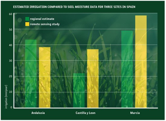
Figure 2. Comparison of observed (statistical survey) and estimated (through satellite soil moisture) annual irrigation volumes for three regions in Spain (adapted from Brocca et al. [97]).
An alternative method, but based on the same premise, i.e., that soil moisture predictions from (some) land surface models do not contain irrigated water, whereas satellite soil moisture retrievals do, was proposed by Zaussinger et al. [100], who estimated the irrigation water use over the Contiguous United States from various coarse-resolution sensors (ASCAT, SMAP, and AMSR2). This approaches the aggregated deviation between the modeled and satellite-observed soil moisture climatology as an irrigation water use estimate. A similar approach was employed by Zohaib and Choi [101] to identify trends of irrigation water amounts worldwide. Irrigation estimates from both studies showed a good correlation with country-level reported irrigation data, though irrigation was systematically underestimated. Notwithstanding the potential of currently available microwave-based soil moisture products, their biggest limitation to the retrieval of accurate irrigation water amounts is the coarse spatial resolution of (most) sensors, i.e., pixel sizes in the order of tens of km. To address this issue, Dari et al. [102] recently exploited 1 km DISPATCH downscaled versions of SMOS and SMAP soil moisture to estimate almost 7 years of irrigation water amounts over an intensely irrigated area in the North East of Spain. Irrigation was retrieved through an improved version of the SM2RAIN algorithm, in which the crop evapotranspiration was estimated according to the FAO model. Comparisons with district-scale benchmark irrigation volumes showed the suitability of the method to estimate actual irrigation amounts, as well as the skill in reproducing the temporal dynamics of irrigation. Zappa et al. [103] developed a framework for the detection and quantification of irrigation based on the TU-Wien S1 soil moisture product at 500 m resolution [91]. Good agreement was found against field-scale irrigation reference data in Northern Germany, both in terms of spatial patterns and temporal dynamics. However, the overall irrigation volumes were generally underestimated as a result of field-specific irrigation systems and management practices, and the longer revisit time of the S1 images (up to a few days) compared to coarse-scale products.
2.3. Gravimetry-Based Methods
While multispectral-based and microwave-based methods rely on remotely sensed estimates of quantities that are driven directly by irrigation (e.g., the soil water content or vegetation transpiration), gravimetric remote sensing may bear more indirect irrigation information. Specifically, gravimetric measurements have been used to derive so-called terrestrial water storage (TWS), which are temporally averaged (typically monthly) water mass change observations of anomalies of the total mass of water stored on and beneath the land surface. Temporal trends in TWS from GRACE data [104,105], for instance, have been linked to heavily irrigated regions of the world caused by human-induced (irrigation) groundwater depletion (e.g., [106]).
The largest caveat of gravimetric remote sensing, however, is its coarse horizontal resolution, which is about 300 km at mid-latitudes [107]. TWS retrievals, therefore, contain many other confounding factors (such as snow, surface water in lakes and rivers, etc.) that need to be removed when attempting to link TWS anomalies to groundwater depletion from irrigation.
This entry is adapted from the peer-reviewed paper 10.3390/rs13204112
This entry is offline, you can click here to edit this entry!