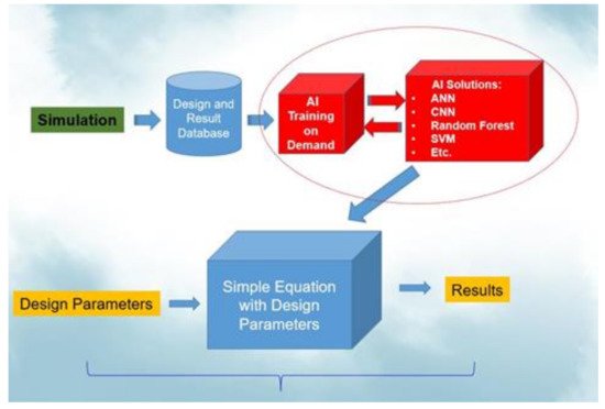
Many researchers have adopted the finite-element-based design-on-simulation (DoS) technology for the reliability assessment of electronic packaging. DoS technology can effectively shorten the design cycle, reduce costs, and effectively optimize the packaging structure. However, the simulation analysis results are highly dependent on the individual researcher and are usually inconsistent between them. Artificial intelligence (AI) can help researchers avoid the shortcomings of the human factor.
- FEM simulation
- WLP
- AI
- machine learning
- ANN
- RNN
- SVR
- KRR
- KNN
- RF
- regression model
1. Introduction
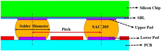
2. Finite Element Method for WLP

| Test Vehicle | Experimental Reliability (Cycles) |
Simulation Reliability (Cycles) |
Difference |
|---|---|---|---|
| TV1 | 318 | 313 | −5 |
| TV2 | 1013 | 982 | −31 |
| TV3 | 587 | 587 | 0 |
| TV4 | 876 | 804 | 72 |
| TV5 | 904 | 885 | 19 |
3. Machine Learning
3.1. Establishment of Dataset
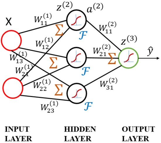
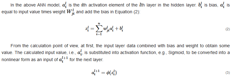
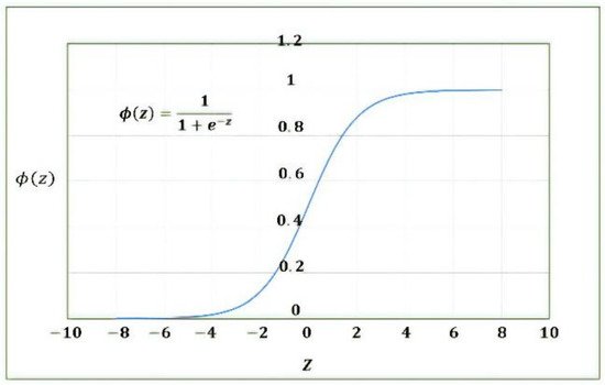
3.2. ANN Model
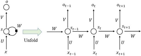
3.3. RNN Model
3.4. SVR Model
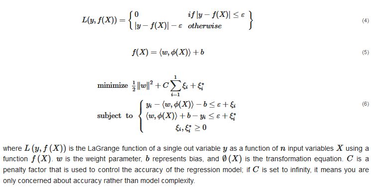
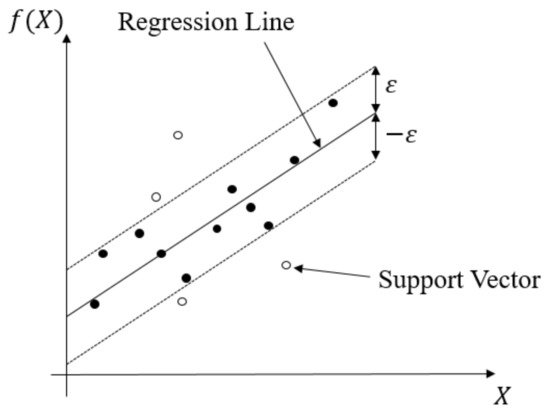
This regression method evolved from the support vector machine algorithm. It transforms data to high-dimensional feature space and adapts the ε-insensitive loss function (Equation (4)) to perform the linear regression in feature space (Equation (5)). In this regression method, the norm value of w is also minimized to avoid the overfitting problem. In other words, f(X,w), which is the function of the SVR model, will be as flat as possible. The SVR concept is illustrated in Figure 10. The data points outside the ε-insensitive zone are called support vectors, and two slack variables, ξi and ξ∗i, are used to record the loss of each support vector. Thus, the whole SVR problem can be seen as an optimization problem (Equation (6)).


3.5. KRR Model
KRR combines ridge regression with the kernel “trick”. This model can learn a linear function in the space induced by the respective kernel and the dataset. Nonlinear functions in the original space can be used by the nonlinear kernels. The KRR algorithm also analyzes several kernels such as the RBF kernel, sigmoid kernel, and polynomial kernel to find the suitable kernel function for the WLP nonlinear dataset.
The KRR is possibly the most elementary algorithm that can be kernelized to ridge regression [31]. The classic method is used to minimize the quadratic cost, as shown in Equation (8). However, for the nonlinear dataset, the lower-dimensional feature space replaces the higher-dimensional feature space; that is, Xi→Φ(Xi). To convert lower-dimensional space to higher-dimensional space, the predictive model undergoes overfitting. Hence, to avoid overfitting, this function requires regularization.
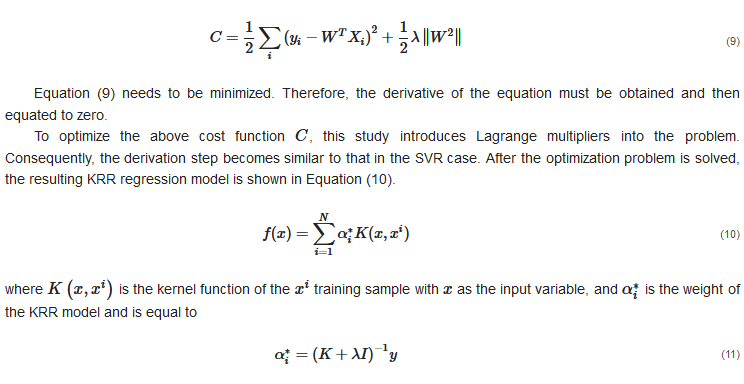
Hence, Equation (11) is very simple and more flexible due to introducing kernel function K, λ is the regularize factor with the identity matrix I, and y is the response variable. This model can also avoid both model complexity and computational time.
3.6. KNN Model
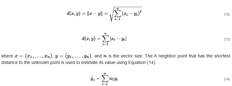
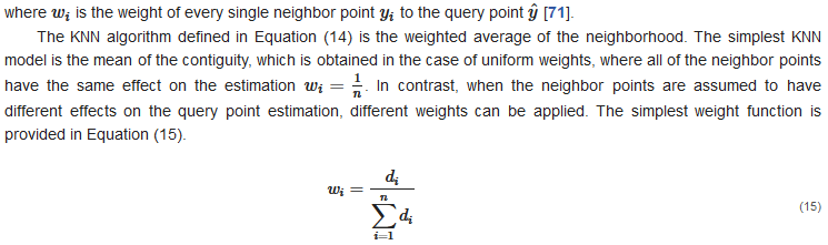
The KNN model is a statistical tool for estimating the value of an unknown point based on its nearest neighbors [69]. The nearest neighbors are usually calculated as the points with the shortest distance to the unknown point [70]. Several techniques are used to measure the distance between the neighbors. Two simple techniques are used in this study: the Euclidean distance function d(x,y), provided in Equation (12), and the Manhattan distance function d(x,y), provided in Equation (13).
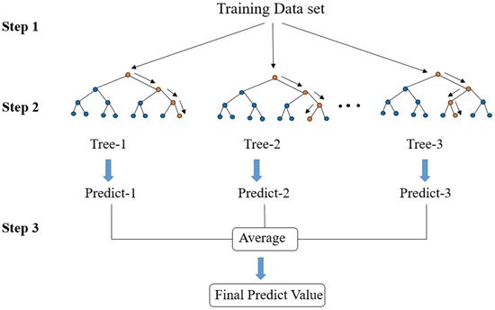
3.7. The RF Regression Model
3.8. Training Methodology
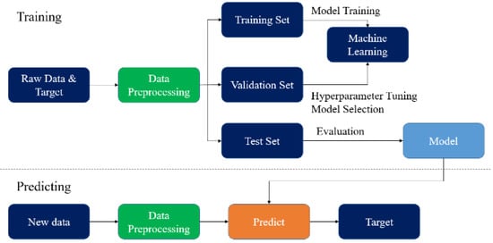
3.8.1. Data Preprocessing
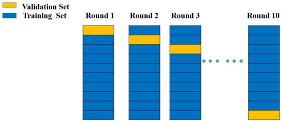
3.8.2. Cross-Validation
3.8.3. Grid Search Technique
This entry is adapted from the peer-reviewed paper 10.3390/ma14185342
References
- Andriani, Y.; Wang, X.; Seng, D.H.L.; Teo, S.L.; Liu, S.; Lau, B.L.; Zhang, X. Effect of Boron Nitride Nanosheets on Properties of a Commercial Epoxy Molding Compound Used in Fan-Out Wafer-Level Packaging. IEEE Trans. Compon. Packag. Manuf. Technol. 2020, 10, 990–999.
- Cheng, H.-C.; Chung, C.-H.; Chen, W.-H. Die shift assessment of reconstituted wafer for fan-out wafer-level packaging. IEEE Trans. Device Mater. Reliab. 2020, 20, 136–145.
- Cheng, H.-C.; Wu, Z.-D.; Liu, Y.-C. Viscoelastic warpage modeling of fan-out wafer-level packaging during wafer-level mold cure process. IEEE Trans. Compon. Packag. Manuf. Technol. 2020, 10, 1240–1250.
- Dong, H.; Chen, J.; Hou, D.; Xiang, Y.; Hong, W. A low-loss fan-out wafer-level package with a novel redistribution layer pattern and its measurement methodology for millimeter-wave application. IEEE Trans. Compon. Packag. Manuf. Technol. 2020, 10, 1073–1078.
- Lau, J.H.; Li, M.; Li, Q.M.; Xu, I.; Chen, T.; Li, Z.; Tan, K.H.; Yong, Q.X.; Cheng, Z.; Wee, K.S. Design, materials, process, fabrication, and reliability of fan-out wafer-level packaging. IEEE Trans. Compon. Packag. Manuf. Technol. 2018, 8, 991–1002.
- Lau, J.H.; Li, M.; Qingqian, M.L.; Chen, T.; Xu, I.; Yong, Q.X.; Cheng, Z.; Fan, N.; Kuah, E.; Li, Z. Fan-out wafer-level packaging for heterogeneous integration. IEEE Trans. Compon. Packag. Manuf. Technol. 2018, 8, 1544–1560.
- Lee, T.-K.; Xie, W.; Tsai, M.; Sheikh, M.D. Impact of Microstructure Evolution on the Long-Term Reliability of Wafer-Level Chip-Scale Package Sn–Ag–Cu Solder Interconnects. IEEE Trans. Compon. Packag. Manuf. Technol. 2020, 10, 1594–1603.
- Zhao, S.; Yu, D.; Zou, Y.; Yang, C.; Yang, X.; Xiao, Z.; Chen, P.; Qin, F. Integration of CMOS image sensor and microwell array using 3-D WLCSP technology for biodetector application. IEEE Trans. Compon. Packag. Manuf. Technol. 2019, 9, 624–632.
- Chen, C.; Yu, D.; Wang, T.; Xiao, Z.; Wan, L. Warpage prediction and optimization for embedded silicon fan-out wafer-level packaging based on an extended theoretical model. IEEE Trans. Compon. Packag. Manuf. Technol. 2019, 9, 845–853.
- Lau, J.H.; Ko, C.-T.; Tseng, T.-J.; Yang, K.-M.; Peng, T.C.-Y.; Xia, T.; Lin, P.B.; Lin, E.; Chang, L.; Liu, H.N. Panel-level chip-scale package with multiple diced wafers. IEEE Trans. Compon. Packag. Manuf. Technol. 2020, 10, 1110–1124.
- Lau, J.H.; Li, M.; Yang, L.; Li, M.; Xu, I.; Chen, T.; Chen, S.; Yong, Q.X.; Madhukumar, J.P.; Kai, W. Warpage measurements and characterizations of fan-out wafer-level packaging with large chips and multiple redistributed layers. IEEE Trans. Compon. Packag. Manuf. Technol. 2018, 8, 1729–1737.
- Qin, C.; Li, Y.; Mao, H. Effect of Different PBO-Based RDL Structures on Chip-Package Interaction Reliability of Wafer Level Package. IEEE Trans. Device Mater. Reliab. 2020, 20, 524–529.
- Qin, F.; Zhao, S.; Dai, Y.; Yang, M.; Xiang, M.; Yu, D. Study of warpage evolution and control for six-side molded WLCSP in different packaging processes. IEEE Trans. Compon. Packag. Manuf. Technol. 2020, 10, 730–738.
- Wang, P.-H.; Huang, Y.-W.; Chiang, K.-N. Reliability Evaluation of Fan-Out Type 3D Packaging-On-Packaging. Micromachines 2021, 12, 295.
- Yang, C.; Su, Y.; Liang, S.Y.; Chiang, K. Simulation of wire bonding process using explicit FEM with ALE remeshing technology. J. Mech. 2020, 36, 47–54.
- Liu, C.-M.; Lee, C.-C.; Chiang, K.-N. Enhancing the reliability of wafer level packaging by using solder joints layout design. IEEE Trans. Compon. Packag. Technol. 2006, 29, 877–885.
- Chiang, K.-N.; Chen, W.-H.; Cheng, H.-C. Large-scale three-dimensional area array electronic packaging analysis. J. Comput. Model. Simul. Eng. 1999, 4, 4–11.
- Tsou, C.; Chang, T.; Wu, K.; Wu, P.; Chiang, K. Reliability assessment using modified energy based model for WLCSP solder joints. In Proceedings of the International Conference on Electronics Packaging (ICEP), Yamagata, Japan, 19–22 April 2017; pp. 7–15.
- Liu, S.; Panigrahy, S.; Chiang, K. Prediction of fan-out panel level warpage using neural network model with edge detection enhancement. In Proceedings of the IEEE 70th Electronic Components and Technology Conference (ECTC), Orlando, FL, USA, 3–30 June 2020; pp. 1626–1631.
- Yuan, C.C.; Lee, C.-C. Solder joint reliability modeling by sequential artificial neural network for glass wafer level chip scale package. IEEE Access 2020, 8, 143494–143501.
- Ramalho, L.; Belinha, J.; Campilho, R. A new crack propagation algorithm combined with the finite element method. J. Mech. 2020, 36, 405–422.
- Chang, J.; Wang, L.; Dirk, J.; Xie, X. Finite element modeling predicts the effects of voids on thermal shock reliability and thermal resistance of power device. Weld. J. 2006, 85, 63s–70s.
- JEDEC Solid State Technology Association. JEDEC Standard JESD22-A104D, Temperature Cycling. Jedec. Org 2005, 11, 2009.
- Coffin, L.F., Jr. A study of the effects of cyclic thermal stresses on a ductile metal. Trans. ASME 1954, 76, 931–950.
- Ramachandran, V.; Wu, K.; Chiang, K. Overview study of solder joint reliablity due to creep deformation. J. Mech. 2018, 34, 637–643.
- Lee, C.-H.; Wu, K.-C.; Chiang, K.-N. A novel acceleration-factor equation for packaging-solder joint reliability assessment at different thermal cyclic loading rates. J. Mech. 2017, 33, 35–40.
- Chou, P.; Chiang, K.; Liang, S.Y. Reliability assessment of wafer level package using artificial neural network regression model. J. Mech. 2019, 35, 829–837.
- Tang, Z.; Fishwick, P.A. Feedforward neural nets as models for time series forecasting. ORSA J. Comput. 1993, 5, 374–385.
- Zhang, D.; Han, X.; Deng, C. Review on the research and practice of deep learning and reinforcement learning in smart grids. CSEE J. Power Energy Syst. 2018, 4, 362–370.
- Gers, F.A.; Schmidhuber, J.; Cummins, F. Learning to forget: Continual prediction with LSTM. Neural Comput. 2000, 12, 2451–2471.
- Welling, M.; Kernel Ridge Regression. Max Welling’s Class Notes in Machine Learning. 2013. Available online: https://web2.qatar.cmu.edu/~gdicaro/10315/additional/welling-notes-on-kernel-ridge.pdf (accessed on 6 August 2021).