The Curiosity rover has landed on Mars since 2012. One of the instruments onboard the rover is a pair of multispectral cameras known as Mastcams, which act as eyes of the rover.
1. Introduction
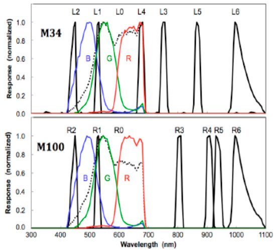
Onboard the Curiosity rover, there are a few important instruments. The laser induced breakdown spectroscopy (LIBS) instrument, ChemCam, performs rock composition analysis from distances as far as seven meters [2]. Another type of instrument is the mast cameras (Mastcams). There are two Mastcams [3]. The cameras have nine bands in each with six of them overlapped. The range of wavelengths covers the blue (445 nanometers) to the short-wave near-infrared (1012 nanometers).
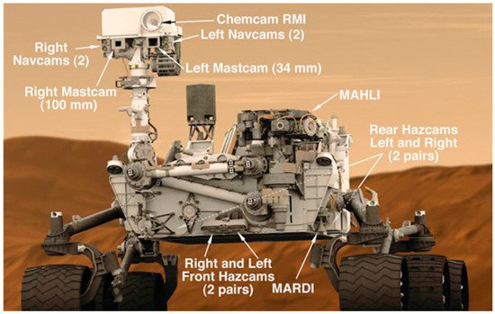
The Mastcams can be seen in
Figure 1. The right imager has three times better resolution than the left. As a result, the right camera is usually for short range image collection and the right is for far field data collection. The various bands of the two Mastcams are shown in
Table 1 and
Figure 2. There are a total of nine bands in each Mastcam. One can see that, except for the RGB bands, the other bands in the left and right images are non-overlapped, meaning that it is possible to generate a 12-band data cube by fusing the left and right bands. The dotted curves in
Figure 2 are known as the “broadband near-IR cutoff filter”, which has a filter bandwidth (3 dB) of 502 to 678 nm. Its purpose is to help the Bayer filter in the camera [
3]. In a later section, the 12-band cube was used for accurate data clustering and anomaly detection.
Figure 1. The Mars rover—Curiosity, and its onboard instruments [
4]. Mastcams are located just below the white box near the top of the mast.
Figure 2. Spectral response curves for the left eye (top panel) and the right eye (bottom panel) [
5].
2. Perceptually Lossless Compression for Mastcam Images
Up to now, NASA is still compressing the Mastcam images without loss using JPEG, which is a technology developed around 1990 [
6]. JPEG is computationally efficient. However, it can achieve a compression ratio of at most three times in the lossless compression mode. In the past two decades, new compression standards, including JPEG-2000 (J2K) [
7], X264 [
8], and X265 [
9], were developed. These video codecs can also compress still images. Lossless compression options are also present in these codecs.
The objective of our recent study [
12] was to perform thorough comparative studies and advocated the importance of using perceptually lossless compression for NASA’s missions. In particular, in our recent paper [
12], we evaluated five image codecs, including Daala, X265, X264, J2k, and JPEG.
Our findings are as follows. Details can be found in [
12].
-
Comparison of different approaches
For the nine-band multispectral Mastcam images, we compared several approaches (principal component analysis (PCA), split band (SB), video, and two-step). It was observed that the SB approach performed better than others using actual Mastcam images.
-
Codec comparisons
In each approach, five codecs were evaluated. In terms of those objective metrics (HVS and HVSm), Daala yielded the best performance amongst the various codecs. At ten to one compression, more than 5 dBs of improvement was observed by using Daala as compared to JPEG, which is the default codec by NASA.
-
Computational complexity
Daala uses discrete cosine transform (DCT) and is more amenable for parallel processing. J2K is based on wavelet which requires the whole image as input. Although X265 and X264 are also based on DCT, they did not perform well at ten to one compression in our experiments.
-
Subjective comparisons
Using visual inspections on RGB images, it was observed that at 10:1 and 20:1 compression, all codecs have almost no loss. However, at higher compression ratios such as 40 to 1 compression, it was observed that there are noticeable color distortions and block artifacts in JPEG, X264, and X265. In contrast, we still observe good compression performance in Daala and J2K even at 40:1 compression.
3. Debayering for Mastcam Images
The nine bands in each Mastcam camera contain RGB bands. Different from other bands, the RGB bands are collected by using a Bayer pattern filter, which first came out in 1976 [
14]. In the past few decades, many debayering algorithms were developed [
15,
16,
17,
18,
19]. NASA still uses the Malvar-He-Cutler (MHC) algorithm [
20] to demosaic the RGB Mastcam images. Although MHC was developed in 2004, it is an efficient algorithm that can be easily implemented in the camera’s control electronics. In [
3], another algorithm known as the directional linear minimum mean square-error estimation (DLMMSE) [
21] was also compared against the MHC algorithm.
Deep learning has gained popularity since 2012. In [
22], a joint demosaicing and denoising algorithm was proposed. For the sake of easy referencing, this algorithm can be called DEMOsaic-Net (DEMONET). Two other deep learning-based algorithms for demosaicing [
23,
24] have been identified as well.
We have several observations on our Mastcam image demosaicing experiments. First, we observe that the MHC algorithm still generated reasonable performance in Mastcam images even though some recent ones yielded better performance. Second, we observe that some deep learning algorithms did not always perform well. Only the DEMONET generated better performance than conventional methods. This shows that the performance of demosaicing algorithms depends on the applications. Third, we observe that DEMONET performed better than others only for right Mastcam images. DEMONET has comparable performance to a method know as exploitation of color correlation (ECC) [
31] for the left Mastcam images.
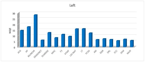
Due to the fact that there are no ground truth demosaiced images, we adopted an objective blind image quality assessment metric known as natural image quality evaluator (NIQE). Low NIQE scores mean better performance. Figure 3 shows the NIQE metrics of various methods. One can see that ECC and DEMONET have better performance than others.
Figure 3. Mean of NIQE scores of demosaiced R, G, and B bands for 16 left images using all methods. MHC is the default algorithm used by NASA.
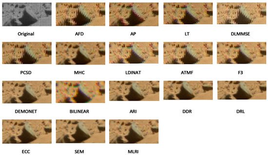
From Figure 4, we see obvious color distortions in demosaiced image using bilinear, MHC, AP, LT, LDI-NAT, F3, and ATMF. One can also see strong zipper artifacts in the images from AFD, AP, DLMMSE, PCSD, LDI-NAT, F3, and ATMF. There are slight color distortions in the results of ECC and MLRI. Finally, we can observe that the images of DEMONET, ARI, DRL, and SEM are more perceptually pleasing than others.
Figure 4. Debayered images for left Mastcam Image 1. MHC is the default algorithm used by NASA.
4. Mastcam Image Enhancement
4.1. Model Based Enhancement
In [
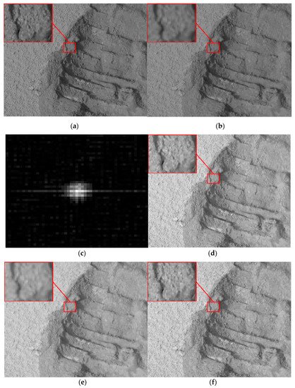
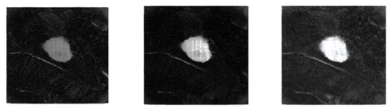
35], we presented an algorithm to improve the left Mastcam images. There are two steps in our approach. First, a pair of left and right Mastcam bands is used to estimate the point spread function (PSF) using a sparsity-based approach. Second, the estimated PSF is then applied to improve the other left bands. Preliminary results using real Mastcam images indicated that the enhancement performance is mixed. In some left images, improvements can be clearly seen, but not so good results appeared in others.
From
Figure 5, we can clearly observe the sharpening effects of the deblurred image (i.e.,
Figure 5f) compared with the aligned left images (i.e.,
Figure 5e). The estimated kernel in
Figure 5c, was obtained using a pair of left and right green bands. We can see better enhancement in
Figure 5 for the LR band. However, in some cases in [
35], some performance degradations were observed.
Figure 5. Image enhancement performance of an LR-pair on sol 0100 taken on 16 November 2012 for L0R filter band aligned image using PSF estimated from 0G filter bands. (a) Original R0G band; (b) L0G band; (c) estimated PSF using L0G image in (b) and R0G image in (a); (d) R0R band; (e) L0R band-PSNR = 24.78 dB; (f) enhanced image of (e) using PSF estimated in (c) PSNR = 30.08 dB.
The mixed results suggest a new direction for future research, which may involve deep learning techniques for PSF estimation and robust deblurring.
4.2. Deep Learning Approach
Over the past two decades, a large number of papers was published on the subject of pansharpening, which is the fusion of a high resolution (HR) panchromatic (pan) image with a low resolution (LR) multispectral image (MSI) [
36,
37,
38,
39,
40]. Recently, we proposed an unsupervised network for image super-resolution (SR) of hyperspectral image (HSI) [
41,
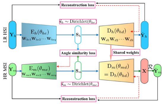
42]. Similar to MSI, HSI has found many applications. The key features of our work in HSI include the following. First, our proposed algorithm extracts both the spectral and spatial information from LR HSI and HR MSI with two deep learning networks, which share the same decoder weights, as shown in
Figure 6. Second, sum-to-one and sparsity are two physical constraints of HSI and MSI data representation. Third, our proposed algorithm directly addresses the challenge of spectral distortion by minimizing the angular difference of these representations.
Figure 6. Simplified architecture of the proposed uSDN.
To generate objective metrics, we used the root mean squared error (RMSE) and spectral angle mapper (SAM), which are widely used in the image enhancement and pansharpening literature. Smaller values imply better performance.
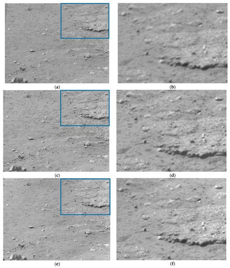
Figure 7 shows the images of our experiments. One can see that the reconstructed image is comparable to the ground truth. Here, we only compare the proposed method with coupled nonnegative matrix factorization (CNMF) [
46] which has been considered a good algorithm. The results in
Table 2 show that the proposed approach was able to outperform the CNMF in two metrics.
Figure 7. Results of pansharpening for Mars images. Left column (a,c,e) shows the original images; right column (b,d,f) is the zoomed in view of the blue rectangle areas of the left images. The first row (a,b) shows third band from the left camera. The second row (c,d) shows the corresponding reconstructed results. The third row (e,f) shows the third band from the right camera.
5. Stereo Imaging and Disparity Map Generation for Mastcam Images
Mastcam images have been used by OnSight software to create a 3D terrain model of the Mars. The disparity maps extracted from stereo Mastcam images are important by providing depth information. Some papers [51,52,53] proposed methods to estimate disparity maps using monocular images. Since the two Mastcam images do not have the same resolution, a generic disparity map estimation using the original Mastcam images may not take the full potential of the right Mastcam images that have three times higher image resolution. It will be more beneficial to NASA and other users of Mastcam images if a high-resolution disparity map can be generated.
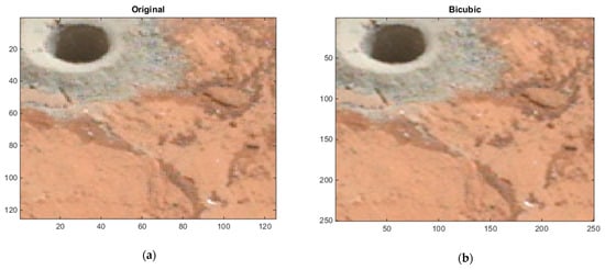
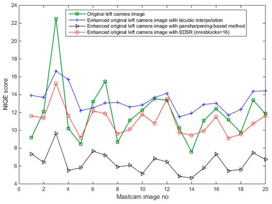
Three algorithms were used to improve left camera images. The bicubic interpolation [56] was used as the baseline technique. Another method [57] is an adaptation of the technique in [5] with pansharpening [57,58,59,60,61]. Recently, deep learning-based SR techniques [62,63,64] have been developed.
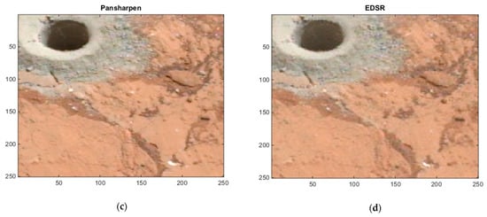
Here, we include some comparative results. From Figure 8, we observe that the image quality with EDSR and the pansharpening-based method are better when compared with the original and bicubic images.
Figure 8. Image enhancements on 0183ML0009930000105284E01_DRCX_0PCT.png. (a) Original left camera image; (b) bicubic-enhanced left camera image; (c) pansharpening-based method enhanced left camera image; (d) EDSR enhanced left camera image.
Figure 9 shows the objective NIQE metrics for the various algorithms.
Figure 9. Natural image quality evaluator (NIQE) metric results for enhanced “original left Mastcam images” (scale: ×2) by the bicubic interpolation, pansharpening-based method, and EDSR.
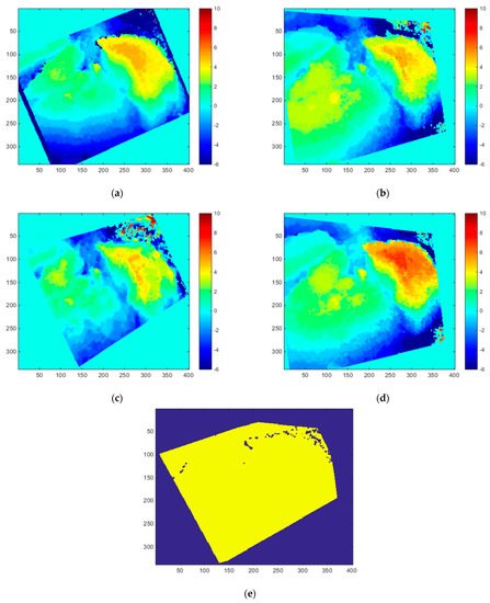
Figure 10 shows the estimated disparity maps with the three image enhancement methods for Image Pair 6 in [
54].
Figure 10. Disparity map estimations with the three methods and the mask for computing average absolute error. (a) Ground truth disparity map; (b) disparity map (bicubic interpolation); (c) disparity map (pansharpening-based method); (d) disparity map (EDSR); (e) mask for computing average absolute error.
6. Anomaly Detection Using Mastcam Images
One important role of Mastcam imagers is to help locate anomalous or interesting rocks so that the rover can go to that rock and collect some samples for further analysis.
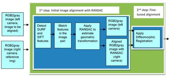
A two-step image alignment approach was introduced in [
5]. The performance of the proposed approach was demonstrated using more than 100 pairs of Mastcam images, selected from over 500,000 images in NASA’s PDS database. As detailed in [
5], the fused images have improved the performance of anomaly detection and pixel clustering applications.
Figure 11 illustrates the proposed two-step approach. The first step uses RANSAC (random sample consensus) technique [
66] for an initial image alignment. SURF features [
67] and SIFT features [
68] are then matched within the image pair.
Figure 11. A two-step image alignment approach to registering left and right images.
tistical method [
70].
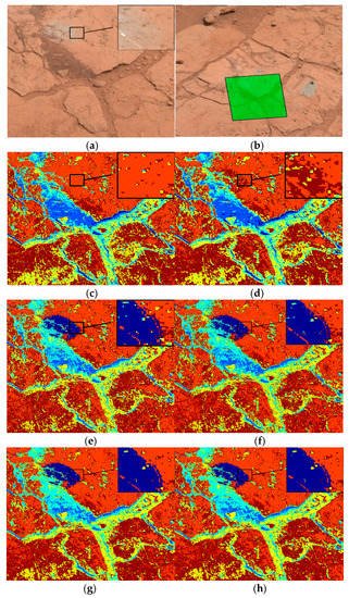
Figure 12 shows the results. In each figure, we enlarged one clustering region to showcase the performance. There are several important observations:
Figure 12. Clustering results with six classes of an LR-pair on sol 0812 taken on 18 November 2014. (
a) Original RGB right image; (
b) original RGB left image; (
c) using nine-band right camera MS cube; (
d) using twelve-band MS cube after first registration step with lower (M-34) resolution; (
e) using twelve-band MS cube after the second registration step with lower resolution; (
f) using twelve-band MS cube after the second registration step with higher (M-100) resolution; (
g) using pan-sharpened images by band dependent spatial detail (BDSD) [
71]; and (
h) using pan-sharpened images by partial replacement adaptive CS (PRACS) [
72].
Figure 13 displays the anomaly detection results of two LR-pair cases for the three competing methods (global-RX, local-RX and NRS methods) applied to the original nine-band data captured only by the right Mastcam (second row) and the five twelve-band fused data counterparts (third to seventh rows).
Figure 13. Comparison of anomaly detection performance of an LR-pair on sol 1138 taken on 10-19-2015. The first row shows the RGB left and right images; and the second to seventh rows are the anomaly detection results of the six MS data versions listed in [
5] in which the first, second, and third columns are results of global-RX, local-RX [
73] and NRS [
74] methods, respectively.
This entry is adapted from the peer-reviewed paper 10.3390/computers10090111