Your browser does not fully support modern features. Please upgrade for a smoother experience.
Please note this is an old version of this entry, which may differ significantly from the current revision.
Subjects:
Others
The capital asset pricing model (CAPM) is an influential paradigm in financial risk management. It formalizes mean-variance optimization of a risky portfolio given the presence of a risk-free investment such as short-term government bonds. The CAPM defines the price of financial assets according to the premium demanded by investors for bearing excess risk.
- beta
- Sharpe ratio
- three-factor model
- momentum
- intertemporal CAPM
- Roll’s critique
- investor heterogeneity
- multifractality
- efficient market hypothesis
- fractal market hypothesis
1. Introduction
The capital asset pricing model (CAPM) is an influential and popular model for describing the price of financial assets such as publicly traded stock. The CAPM traces its origins to “general models” seeking to solve “the problem of capital asset pricing under uncertainty” [1] (p. 40). The CAPM assumes that investors are risk-averse and demand additional return as compensation for bearing risk. Like most other aspects of mathematical finance, the CAPM implicitly endorses the rational expectations hypothesis [2]. The CAPM presumes that rational, welfare-maximizing agents will understand and act upon an “objective probability law” that quantifies the relationship between risk and return [3] (p. 283).
An efficient market rewards the assumption of risk by investors with higher returns [4]. The fundamental expectation that returns in excess of a risk-free baseline “should vary positively and proportionately to market volatility” is properly regarded as the “first law of finance” [5] (p. 233). The Supreme Court of the United States has offered a simpler formulation: “The less risk, the less right to any unusual returns upon … investments” [6] (p. 49).
Section 2 of this entry derives the CAPM from its origins in mean-variance optimization, the basis of modern portfolio theory. It describes the Treynor and Sharpe ratios. Section 3 focuses on beta, the mathematical building block for many variants of the CAPM. Section 4 harmonizes the CAPM with asset-pricing theories distinguishing quantifiable risk from complete uncertainty. Section 5 identifies and discusses practical applications of the CAPM. Section 6 recounts criticisms of the CAPM. Section 7 elaborates the extension of the CAPM to account for multifractality in volatility. Section 8 explains why the CAPM persists despite blows to its empirical underpinnings.
2. Deriving and Defining the Capital Asset Pricing Model
2.1. Mean-Variance Optimization and the Tangency Portfolio
The seductively simple CAPM “offers powerful and intuitively pleasing” explanations for the relationship between risk and return [7] (p. 25). The capital asset pricing model extends the exercise of mean-variance optimization at the heart of modern portfolio theory [8]. Mean-variance efficient portfolios minimize variance for any expected return. Given a level of variance, efficient portfolios maximize return.
Figure 1 illustrates the derivation of the CAPM from a schematic depiction of mean-variance optimization [9] (p. 139). Figure 1 represents expected return on investments within a portfolio as a function of risk. The horizontal axis reports risk as measured by some surrogate such as the standard deviation or the beta of portfolio returns. An investor seeking to maximize return must accept higher variance.
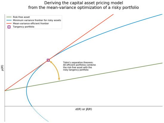
Figure 1. Deriving the CAPM from the mean-variance optimization of a risky portfolio.
The blue parabola in Figure 1 shows the relationship between return and risk in quadratic terms. An investor contemplating the risky market may presumably elect to hold a risk-free asset. At the tangency point, the investor maximizes the ratio of expected return to standard deviation or beta [10][11][12][13]. According to Tobin’s separation theorem, all efficient portfolios combine the risk-free asset with the risky tangency portfolio [14]. Returns on those efficient portfolios, visualizable as linear slopes, therefore range between the risk-free rate and the return on the market-wide tangency portfolio.
2.2. Defining the Risk Premium and the Risk-Free Rate through the Securty Market Line
The CAPM quantifies the market premium for shouldering risk in an asset in excess of a benchmark represented by the return on a risk-free investment. In the original formulation of the CAPM [10][11], return on any asset within the optimized tangency portfolio is expressed in terms of standard deviation (also called “volatility” throughout the literature of finance):
 where ra, rm, and rf represent returns on the asset, the broader market, and the risk-free baseline (respectively), and where σa represents the individual asset’s volatility relative to the whole market. This formula takes the form of a linear function that defines return on an asset (ra) in terms of its volatility (σa).
Because real-world investors may struggle to borrow and lend without restrictions, one version of the CAPM achieves mean-variance optimization through unrestricted short-selling of risky assets [15] (pp. 452–454). The most familiar formulation of the CAPM, however, retains the assumption that the presence of a risk-free asset enables investors to borrow and lend freely. This variant’s primary innovation lies in its expression of the CAPM in terms of beta [16] (p. xv):

So expressed, the CAPM assumes the canonical form of a linear equation, y = b + mx. Plotting asset return (ra) against beta (βa) reveals the security market line [17]. Figure 2 depicts the security market line. Its slope indicates the risk premium (rm − rf), and its intercept is the risk-free return (rf). Permitting “riskless lending opportunities changes the nature of the market equilibrium in just one way …. The expected return on a security continues to be a linear function of its β” [15] (p. 454).
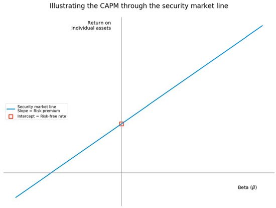
Figure 2. The security market line represents the CAPM as a linear function.
2.3. The Treynor and Sharpe Ratios
The Treynor ratio summarizes the CAPM as specified according to beta [18] (p. 941):

Substituting volatility for beta in the denominator yields the Sharpe ratio [19][20][21]. The Sharpe ratio closely resembles the definition of a z-score in statistics (z=x−μσ):

On the left side of Equations (3) and (4), the term rm−rf indicates the difference between returns on a specific investment or class of investments and the risk-free baseline. This risk premium, derived from variability in an asset’s performance over time, dictates a firm’s cost of capital [22] (p. 262). The CAPM therefore guides corporate capital budgeting amid financial uncertainty [11] (pp. 28–33).
3. Beta
Beta’s prominence in the theoretical literature and in practical applications of the CAPM justifies a closer look at the basic unit of financial co-movement [23], By expressing covariance between a single security and the whole market, beta supplies the simplest measure of systematic risk not reducible through diversification [24] (p. 281). Beta accordingly supplies information on volatility and liquidity throughout the market.
3.1. Correlated Relative Volatility
For any two sets of returns, x and y, beta for y is the ratio of the covariance between the two sets of returns to the variance of x [25] (p. 565):

In many applications, beta compares returns on a single asset or an asset class with returns on the tradable universe.

3.2. Interpreting Beta: Systematic Versus Idiosyncratic Risk
Despite its definition as correlated relative volatility, beta differs from each of its components. Beta is less comprehensive than standard deviation, which captures both systematic and idiosyncratic risk. Beta is arguably more useful in signaling success in portfolio management, since it can isolate forecasting skill from dumb luck or a manager’s risk appetite.
Unlike standard deviation, beta can be negative. Unlike correlation, beta does not range strictly between −1 and +1. Though beta has no upper or lower bound, useful benchmark can be found at β ≈ −1, 0, and +1. Zero beta indicates an absence of correlation between an asset and its benchmark. Negative beta indicates inverse correlation. Positive market movement for an asset with negative beta generates a loss in value. By contrast, such an asset gains value when the broader market declines.
Most applications of beta involve positive values. This resets the analytical baseline to β ≈ +1. Beta of +1 indicates an asset whose systematic volatility responds precisely to movements in the broader market. Where 0 < β < 1, the relevant asset moves in the same direction as the market, though with less sensitivity. Beta exceeding 1 indicates greater sensitivity to market-wide movements.
Certain assets seek negative beta. The canonical example is an inverse exchange-traded fund that uses derivatives to hedge against a decline in the broader market. This inverse ETF seeks a beta of −1 relative to the Standard & Poor’s 500 index. Such an ETF offsets losses from a broader market decline without short-selling.
Under peculiar circumstances, zero beta may fail to signal rampant volatility in a particular asset or asset class. Such miscalibration may arise through a complete lack of correlation with the market. Even for an asset that is turbulent in absolute terms, zero correlation with market-wide trends yields zero beta [28] (p. 1361). Naked speculation in cryptocurrency, for instance, may generate wild swings unconnected with prices on other assets [29]. Beta would fail to detect the palpable risk reported by uncorrelated standard deviation. Mathematically speaking: β ≈ 0; σ ≫ 0.
4. Information Uncertainty and Higher-Moment CAPM
4.1. Risk Versus Uncertainty
The CAPM can be harmonized with more sophisticated theories of asset pricing. All financial models seek to describe how investors respond to uncertainty and to predict how investor behavior will ultimately drive capital asset prices. Many models falter, however, where “risks are not well understood, where the range of outcomes is potentially very large, and where probabilities cannot be assigned with confidence” [30] (p. 906). The question is whether the CAPM can accommodate the theoretical distinction between quantifiable risk and wholly unknowable uncertainty.
The accommodation of risk and uncertainty as distinct facets of asset pricing has deep roots in the history of economic thought. Frank Knight distinguished between “risk” as “a quantity susceptible of measurement” and the “radically distinct” concept of “uncertainty” of a “nonquantitative type” [31] (pp. 19–20). With respect to some questions, John Maynard Keynes acknowledged, “there is no scientific basis on which to form any calculable probability whatever” [32] (p. 213).
More formally, risk refers to unknown outcomes within a known distribution, while uncertainty describes circumstances where the distribution of outcomes is wholly unknown [5] (p. 234). In practical terms, quantifiable risk characterizes situations where “probabilities are available to guide choice,” while purely aleatory uncertainty describes circumstances in which “information is too imprecise to be summarized by probabilities” [3] (p. 283).
4.2. Information Uncertainty
Uncertainty arising from “ambiguity with respect to … new information for a firm’s value” can disrupt capital markets [33] (p. 105). Information uncertainty exacts a particularly steep toll in declining markets. Whether it is attributable to events affecting a specific firm or industry or reflective of effects in the broader economy, retrenchment cripples the flow of information through trading and other forms of business activity [34] (p. 162).
Investors “prefer to act on known rather than unknown or vague probabilities” [3] (p. 284). When informational “quality is difficult to judge, investors treat signals as ambiguous” [35] (p. 197). As ambiguity amplifies uncertainty, investors lose the ability to evaluate the risk of default, the magnitude of default-related losses, the default premium, and deadweight loss from business failure [36]. The premium associated with all of these forms of uncertainty will rise sharply.
As it compounds the burden from other investment-related risks, information uncertainty can leave a deep footprint on asset prices. When they face uncertainty over “the correct probability laws governing the market return,” investors “demand a higher premium to hold the market portfolio” [5] (p. 234). That response is consistent with conventional understandings of the CAPM as a model of investor behavior.
4.3. Generalizing the CAPM to Accommodate Both Risk and Uncertainty
Equation (7) formally expresses the relationship between risk and uncertainty [5] (pp. 233–234):

In Equation (7), E designates the expectation operator. The variable re indicates excess return over the risk-free baseline. V indicates market-wide conditional volatility, and M measures uncertainty throughout the economy. The temporal indexing variable t governs all of these variables as well as the expectation operator.
Coefficients γ and θ indicate aversion, respectively, to risk and uncertainty. Positive values for both coefficients imply that “both risk and uncertainty carry a positive premium” [5] (p. 234). If an investor is wholly indifferent to uncertainty (so that θ = 0), or if there is no uncertainty (so that case M = 0), expected return becomes a linear function of volatility alone, or γVt. Elimination of the uncertainty term would recover the conventional CAPM as a special case of the more general asset-pricing formula in Equation (7).
4.4. Higher-Moment CAPM
The separate designation of probabilistic risk and aleatory uncertainty as distinct quantities invites the extension of the conventional CAPM into a higher-moment variant. Mean and variance, after all, represent the first two moments of the probability distribution of logarithmic returns. As long as higher moments are finite—something that cannot be taken for granted if returns follow a stable Paretian distribution and therefore exhibit infinite variance and perhaps even pathologically indeterminant higher moments [37][38]—the CAPM can be expressed in terms of skewness and kurtosis in addition to mean and variance [39][40][41][42].
The Taylor series expansion of log returns can approximate the expected utility function for a portfolio of assets in a form compatible with the canonical CAPM [41] (pp. 469–470); [43] (p. 33). If the logarithm of continuously compounded returns is expressed as f(x)=ln(1+x), then taking the Taylor series expansion of f(x) at x = µ yields:
 where o[(x−μ)5] represents remaining terms of the fifth order and above [44] (p. 11); [45] (p. 1269).
Modest assumptions such as “positive marginal utility, decreasing risk aversion,” and “strict consistency” in attitudes regarding the direction and dispersion of returns without regard to wealth make it easy to interpret this higher-moment asset pricing model [43] (p. 33). The alternating pattern of plus and minus signs indicates that Investors prefer high values for odd-numbered moments (mean and skewness), but low values for even-numbered moments (variance and kurtosis) [46][47]; [48] (p. 917). Lottery-like gains on the upside are attractive, whereas uncertainty over the dispersion of returns, especially on the downside, is repellant [39] (p. 1336); [40] (p. 241).
5. Applications of the CAPM
Because the CAPM applies to portfolios as well as individual securities, its applications abound. Companies, investors, portfolio managers, and even governmental officials can all deploy the CAPM. This section discusses three specific applications: the regulatory CAPM, the model’s use in measuring performances by investment portfolios and their managers, and the CAPM as a guide to asset allocation and investment planning.
5.1. The Regulatory CAPM
A legally significant application of this model is the regulatory CAPM. Regulators can use the CAPM to determine the cost of capital for a shareholder-owned utility company. The Florida Public Service Commission, for instance, uses a utility-specific, regulatory variant of the CAPM to calculate the cost of equity for water and wastewater utilities [49] (p. 89):
 where the subscript u not only indicates the rate of return required to attract investors (ru), but also measures risk borne by comparable firms engaged in the transport of water and wastewater (βu) [50] (pp. 692–693). As is evident from its formulation and the law’s simultaneous solicitude for firm revenue and investor reward, the regulatory CAPM reflects the model’s dual functionality as a gauge of firm-specific and market-wide risk and return.
5.2. Measuring Portfolio and Managerial Performance
5.2.1. The Sharpe Ratio
One of the most popular applications of the CAPM arises directly from the model’s derivation from mean-variance optimization of the risky tangent portfolio. The Sharpe ratio can report how well returns from an equity portfolio track a broad index such as the S&P 500 [51] (p. 10). Such a comparison reveals the equity risk premium.
5.2.2. Jensen’s Alpha
The beta-specified version of the CAPM gives rise to an even more explicit measure of success in portfolio management. The time-series regression of returns generates an intercept term as well as an error term [55] (pp. 393–394):
 where the subscript π designates values associated with an actively managed portfolio. Like the CAPM itself, this formula assumes linear form (Figure 3).
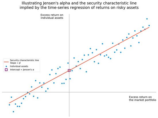
Figure 3. The security characteristic line and Jensen’s α.
The CAPM implies that the beta term should explain the equity premium. Therefore, any upward departure from presumptive intercept of zero represents a positive value for “Jensen’s alpha” or “the average incremental rate of return on the portfolio … due solely to the manager’s ability to forecast future security prices” [55] (p. 394).
5.3. Asset Allocation and Financial Planning
5.3.1. Bond Allocations
Applications of the CAPM emphasizing the performance of investment portfolios and managers imply that the model can also inform investment decisions from the perspective of an individual or institutional investor. Popular investment advice urges risk-averse investors to seek shelter in bonds. Ref. [56] argued that this popular advice contradicts the CAPM because it violates the separation theorem, which provides that all investors should hold the same risky portfolio and rely exclusively on cash or borrowing at the risk-free rate to manage risk [14][57].
In fairness, one branch of popular investment advice, heavily influenced by the CAPM and its theoretical apparatus [58], does urge investors to favor bad companies as good stocks [59] (p. 174); [60] (pp. 548–558); [61] (p. 392). Building a portfolio in line with this advice would raise not only the portfolio’s risk, but also the value of effective diversification.
Closer examination of the relationship of mean to variance for all asset classes rehabilitates the CAPM as a crude but popular basis for asset allocation and investment planning. Stocks are indeed risky, and returns on cash are not enough to compensate some investors [62]. Heterogeneity among investors holds the key: “it is impossible to find better portfolios for all risk-averse investors” [62] (p. 1006). As a matter of financial theory, the existence of different levels of risk aversion among investors vindicates popular advice on the use of bonds to diversify stock holdings [63] (pp. 1178–1179).
5.3.2. Defined Benefit and Defined Contribution Pension Plans
The CAPM informs financial planning for a wide range of individual and institutional investors. Benchmarking to an index, the logical consequence of William Sharpe’s critique of active management [54], gives rise to a bifurcated CAPM distinguishing between indexed returns and the risk/return profile of active managers working on behalf of institutional investors [64].
Perhaps the most intense version of this application involves defined benefit pension plans and the very high probability that large, company-specific or multiemployer plans will default and transfer their liabilities to the Pension Benefit Guaranty Corporation [65] or its equivalent outside the United States [66][67]. For defined contribution plans, which transfer investment risk to employees as individual investors, the CAPM supplies the analytical power behind mean-variance dynamic optimization [68][69][70].
Challenges in asset allocation highlight weaknesses in the CAPM. Among other sources [71][72], Menoncin and Vigna acknowledge that “mean-variance portfolio selection is a time-inconsistent problem due to the presence of the variance of final wealth” [68] (p. 126). Crippled by unrealistic assumptions about time, sources and uses of wealth, and differences among investors, the conventional CAPM struggles to offer sound, reliable financial advice. Difficulties faced by pension administrators and other investors therefore set the stage for criticisms of the CAPM—and may even pave the path toward improving the model.
6. Criticisms of the CAPM
At their most cynical, historians and philosophers of science assert “that the eminence of a scientist is measured by the length of time that he holds up progress in his field” [73] (p. 70). By that benchmark, the CAPM is one of the most eminent landmarks in financial economics. Key elements of this discipline have arisen from efforts to discredit the capital asset pricing model.
Criticisms of the CAPM fall into two broad classes. Waves of empirical discovery of asset-pricing anomalies not satisfactorily explained by beta would eventually generate multifactor alternatives to the CAPM. Categorical exceptions to the conventional CAPM, particularly those based on value, size, and momentum, would populate the “factor zoo”.
A second class of criticisms preserves the mathematical underpinnings of the mean-variance framework, but uses quantitative methods to overcome the limitations of the conventional CAPM. Higher-moment CAPM, addressed in Section 4.4 of this Entry, may be regarded as an instance of this approach.
Other extensions go beyond the expansion of the CAPM to higher statistical moments. They challenge many of the model’s fundamental assumptions. Early critics addressed temporal and spatial limits on the CAPM. Extensions such as the intertemporal CAPM, the consumption-based CAPM, and the evolutionary CAPM epitomize this approach. A focus on informational and behavioral heterogeneity among investors would eventually give rise to multifractal models grounded in complexity theory and econophysics [74][75].
This section reviews the “factor zoo” and basic quantitative extensions of the conventional CAPM. Section 7 will examine multifractality in greater depth.
6.1. Value, Size, and Momentum: The “Factor Zoo”
The quest for asset pricing factors beyond beta originated in Fama and MacBeth’s extension [76] of Jensen’s interpretation [55] of the CAPM as time-series regression. If additional variables in the regression of the cross-section of returns generate slopes statistically distinct from beta, then these variables have identified a factor not incorporated within the canonical CAPM. Using squared market betas as an additional variable, Fama and MacBeth failed to demonstrate a nonlinear relationship between beta and expected return. Nor did Fama and MacBeth uncover heteroskedasticity in residual variances, which would have immediately revealed the presence of predictive variables beyond beta.
Empirical tests of the CAPM have undermined the relationship between beta and expected returns. Anomalous stock pricing associated with the earnings-price ratio [77], the debt-equity ratio [78], and the ratio of book value to market value [79] all indicated a value premium. Lower prices on stocks relative to earnings suggest the presence of other risks [80], later identified as costly reversibility and the countercyclical price of risk [58]. Other sources isolated a distinct size premium associated with smaller firms [81][82]. Subsequent work has cast doubt on the persistence of a size premium [83].
In their grand synthesis of the value and size premiums, Eugene Fama and Kenneth declared that “the relation between β and average return … is weak, perhaps nonexistent” [84] (p. 464). The iconic Fama–French “three-factor” model combines value and size effects with beta [85][86][87]. It describes markets outside the United States [88][89].
Other scholars have identified a fourth factor. Momentum in short-run gains or losses affects stock returns in ways that cannot be ascribed to value or size [90][91][92][93]. The so-called Fama–French–Carhart four-factor model places momentum alongside value, size, and beta [94]. Fama and French have accepted this extension to their three factors [89][95].
Fixed-income market indicators represent an especially fertile source of other candidates for inclusion in factor-based models of asset pricing. Trading in United States Treasury bills, notes, and bonds draws analytical attention to dividend yield, the yield curve as a whole, the term spread, and the default spread on instruments issued by private companies and foreign governments relative to U.S. government securities as presumptively risk-free investments [96].
The rise of factor-based models should be regarded as complementing or extending conventional asset-pricing theories. Amid chaotic efforts to tame these variables within the “factor zoo” [97] (p. 1047), [98], beta and the original CAPM continue to provide “a reasonable ‘first approximation’” for market returns at equilibrium [99] (p.324). The factor zoo, therefore, should not be treated as a comprehensive substitute for the CAPM.
6.2. Relaxing Temporal and Spatial Constraints
6.2.1. The Intertemporal CAPM
The original CAPM assumed that investors hold stock for exactly one period. Moreover, traditional formulations focused almost exclusively on liquid securities listed on markets such as the New York Stock Exchange, NASDAQ, or their equivalents outside the United States. These assumptions cramped the CAPM not only in terms of time, but also in terms of financial space.
By suspending the unrealistic assumption that investors retain stock for exactly one period, the intertemporal capital asset pricing model relaxes the temporal constraint [100]. The time-variant model of asset pricing presented in Section 4.2 and Section 4.3 of this Entry adopts the assumptions of the intertemporal CAPM [3][5][33][35][36]. The desire to preserve (or elevate) current levels of consumption can affect the composition of the market portfolio [100] (p. 877). Assets that retain their value during “innovations … in market volatility” may induce investors to “lower [their] required returns” [101] (p. 64). Paired with more realistic assumptions about heterogeneity in investors’ knowledge and subjective preferences (including risk aversion), the intertemporal CAPM continues to provide the foundation for dynamic time-varying approaches to capital asset pricing [102][103].
6.2.2. Roll’s Second Critique
The concept of financial space may be best understood as the breadth of asset classes available to an investor and covered by a pricing model. Richard Roll’s second critique recognized that investment sets extend beyond publicly traded stocks and include, at a minimum, “bonds, human capital, and real estate” [104] (p. 155). The breadth of the true portfolio suggests that empirical tests do not directly test the CAPM, but rather its validity with respect to a limited proxy such as publicly listed stocks [104] (pp. 154–155), [105]. Indeed, efforts to extend the CAPM to bonds, real estate, and consumer durables have faltered because the volatility of those proxies is dominated by stock market volatility [106].
Despite these challenges, expanding the CAPM beyond its original constraints enables the model to consider human capital and other assets whose value ebbs and flows over a more realistic investment horizon [107]. So modified, the CAPM can serve as the basis for pricing and valuation of any asset over a lifetime or any other timeframe. Indeed, intertemporal differences underlie most of the criticisms and modifications of the CAPM discussed in the balance of this Entry.
6.3. Consumption-Based CAPM
The unpleasant prospect that an investment portfolio might fall short of some minimum level vexes all forms of financial risk management [108]. The consumption-based CAPM addresses this concern. This variant of the capital asset pricing model unites Merton’s intertemporal perspective with the insight that all assets in an exchange economy, in form of stock or otherwise, are ultimately destined to be consumed [109][110][111][112].
A keen desire to safeguard “aggregate real consumption” drives the ideal consumption-based CAPM toward developing “an instantaneously additive price index” that embraces all sources of potential future consumption [109] (p. 267). As each investor “decide[s] how much to save and how much to consume and what portfolio of assets to hold,” the consumption-based CAPM holds that each “asset’s price should equal the expected value of the asset’s payoff” according to “the investor’s marginal utility” [113] (p. 5).
Consistent with other variants of the CAPM, the first-order condition for the consumption-based CAPM “can … be expressed in terms of excess return between … a risky asset k and a risk-free asset f”:
 where Et indicates the expectation at time t and mh, t+1, or the stochastic discount factor, denotes the marginal rate of substitution for individual h between t and t + 1 [114] (p. 449). Beta in this consumption-oriented formulation indicates variability or uncertainty in consumption from holding risky asset k.
Despite being heralded as “one of the major advances in financial economics” during its time [115] (p. 2863), the consumption-based CAPM fared no better than the static, portfolio-based CAPM in empirical tests of its power to explain stock returns [116] (p. 260). Indeed, in many respects, consumption-based CAPM performed worse [115] (p. 2863). In its canonical formulation, consumption-based CAPM has been rejected on the basis of American [117][118] and international data [119].
Later formulations restored some of this model’s explanatory power. In studies of American [114] (pp. 452–459) and global data [120] (p. 2154), consumption-based CAPM fared better once it relaxed the assumption of a homogeneous “representative agent” in favor of heterogeneous agents. This breakthrough invites closer scrutiny of heterogeneity in asset pricing models.
6.4. Modeling Heterogeneous Agents
6.4.1. From Heterogeneity to Heterodoxy
Rejection of the conventional CAPM’s assumption of a homogeneous market of fully rational agents decouples this pillar of financial economics from the efficient market hypothesis [121]. Fittingly enough, the introduction of investor heterogeneity into asset pricing has sparked a diverse profusion of theories. Heterogeneity, as it were, is the mother of heterodoxy.
The simplest theories of heterogeneity rely purely on informational differences. A few traders, either specialists [122] or (more nefariously) insiders [123][124], may obtain superior information. Differences in investor knowledge might be stochastically distributed [125].
One strain of the literature on heterogeneity, however, directly addresses questions of capital asset pricing [126][127][128][129]. This approach to heterogeneity differs from that of later literature elaborating the consumption-based CAPM, which emphasizes low rates of stock market participation among households fitting particular demographic characteristics [114][120]. A distinct literature on the equity market participation puzzle seeks to explain differing rates of exposure to equity investments [130][131].
Despite relaxing one of the assumptions of the conventional CAPM, the introduction of investor heterogeneity preserves certain elements of asset pricing orthodoxy even as it invites theoretical innovation. The segmentation of a market between traders following divergent theories of welfare maximization—namely, expected utility and cumulative prospect theory [132]—nevertheless preserves the security market line, one of the signatures of the conventional CAPM [133]. By the same token, dividing traders into distinct cohorts of arch-rational “fundamentalists” and technical “trend followers” yields an ambitious evolutionary CAPM “characterized by significantly decaying autocorrelation, and positive correlation between, price volatility and trading volume” [134] (p. 185).
6.4.2. Behavioral Capital Asset Pricing
The idea of a behavioral CAPM is broad enough to encompass differences in equity market participation, market segmentation according to divergent definitions of utility, and evolutionary asset pricing theory. Behavioral theories of finance arise through heterogeneity between informed traders and “noise traders,” broadly defined as other parties trading on some basis besides strict rationality [135]. A “market composed solely of information traders” is a market adhering to “price efficiency and the CAPM,” a market where “[r]isk premia are determined solely by beta and the distribution of returns on the market portfolio” [136] (p. 323).
Empirical questions remain. It is one thing to posit differences separating rational information traders from more reactive trend followers [134]. It is another to devise and deploy empirical tests for detecting heterogeneity. The discovery of power law behavior in markets connects behavioral accounts of evolutionary asset pricing and segmented markets with multifractality and the fractal market hypothesis [137][138][139][140]. The next section addresses this step in the continuing evolution of the capital asset pricing model.
7. Multifractality and the Fractal Market Hypothesis
7.1. Beyond Homogeneous Agents and Efficient Markets
The embrace of heterogeneity among investors explicitly rejects the assumptions underlying the canonical CAPM. Key elements of the model’s conventional formulation, particularly the security market line [17] and the separation theorem [14][57], assume that all investors perceive the market portfolio and its constituent assets identically. Such uniformity within the frame of perception persists even if investors select different points along the efficient frontier in order to accommodate idiosyncratic consumption preferences or levels of risk aversion. This degree of homogeneity undergirds the efficient market hypothesis as a supporting pillar of the CAPM [141][142][143][144].
The entire enterprise of behavioral finance (and behavioral economics more generally) rests upon the realization that agents are neither rational (in the classical sense of Homo economicus [145][146]) nor homogeneous. Although many of the efforts to relax the assumption of homogeneity depicted in Section 6.4 have proceeded on differences in access to information or frames of mind, a more appealing and empirically verifiable approach may lie in an extension of the intertemporal CAPM [100]. The very presence of life-cycle effects suggests that rationality for any one individual, even if rigidly and coherently ordered at any one particular moment, might vary during that agent’s lifetime [107].
Multifractal approaches rest on the intuition that heterogeneity may arise from differences in temporal investment horizons, either among investors or even within an individual agent, as circumstances, investment objectives, or entire capital markets evolve [147]. Specifically, the scaling of financial phenomena across time holds the key, not only to the theoretical understanding of heterogeneity, but also to its empirical measurement.
7.2. Volatility, Fractality, and the Generalized Hurst Exponent
Among the basic statistical elements of the canonical CAPM, variance and volatility prove far less tractable than the mean. Volatility ((the financial term of art for standard deviation, or the square root of variance) cannot be directly observed in real time. Historical measures of volatility suffer in two respects: Not only are they purely retrospective, but they also depend entirely on the time horizon. Options pricing provides another imperfect surrogate. Implied volatility may be derived from markets such as VIX [148][149].
The clustering of volatility implies memory in absolute returns over long time horizons [150]. This observation casts doubt on the entire ARCH-GARCH family of volatility models [151][152][153]. Though these approaches recognize autocorrelation in volatility across multiple time steps, they also presume exponential decay [150]. That presumption is incompatible with the persistence of memory.
A process X(t) with uniform increments of τ is fractal if it follows this scaling law:
 where angle brackets ⟨⟩ indicate the expectation and Cq is a constant [154] (p. 026103-1); [155] (p. 6471). “When the exponents ζq are linear in q, a single scaling exponent H is involved,” and the process is monofractal [153] (p. 026103–1). On the other hand, “[i]f the function ζq is no longer linear in q” then process X(t) is multifractal [153] (p. 026103–1); [155] (p. 6471). The special case of H = 0.5 indicates either the complete absence of autocorrelation or a time series for which the absolute value of correlations decay exponentially and quickly to zero [150] (p. 144).
Applications emphasizing the difference between the time and frequency domains distinguish between the scaling of time and the fractality of frequency. Cardiology is a natural example [156][157]. By contrast, some sources in econophysics appear to use the terms multiscaling and multifractal interchangeably to describe volatility as a function of financial time divided into fixed intervals of τ [150][155].
Financial sources also speak of scaling function ζq in terms of the generalized Hurst exponent H(q), such that ζq=qH(q) [158][159][160][161][162]. Nonlinearity in H(q) implies nonlinearity in ζq and a multifractal process. Consistent with sources that use the Hurst exponent to describe structure over longer periods while reserving other representations of fractal dimension for shorter periods [163], sources such as [155] distinguish between possibly “spurious statistical fluctuations” attributable to noise or small sample size and “true structural changes in the underlying multifractal process” (p. 6471).
Amid a sea of diverse empirical methods for detecting and describing multifractality [164], Ladislav Kristoufek has devised various methods of fractal regression [165][166][167][168] for testing the “fractal market hypothesis [74][75][169][170][171]. Multifractality “offers a simple behavioral interpretation” for heterogeneity: Examining “volatility at different timescales is a very natural way to assess the impact of heterogeneous agents” [155] (p. 6470). Indeed, “any measure of scaling behaviour can convey information about the efficiency of a given market” [155] (p. 6470).
7.3. Applications and Implications of Multifractal Analysis
Multifractal analysis of financial markets does more than transform analysis of time-varying volatility and other statistical properties of financial series into a theoretically and empirically satisfying account of investor heterogeneity [172]. It also promises to unite accounts of financial behavior with other multifractal aspects of human conduct, including motor control [173]. In this sense, econophysics converges with the metaphysics of behavioral finance and the “psychophysics of chances” [174] (p. 344).
Multifractal analysis extends the CAPM and its quantitative underpinnings in directions beyond mainstream economics. For example, exploring multifractality across different timescales has the intended effect of revealing investor heterogeneity [175][176]. This method is especially useful in describing heterogeneity across national boundaries, since it reveals differences in investment horizons [176][177]. A comparison of four formerly Communist countries, for instance, aligned Chinse and Czech markets more closely with Germany as a mature market benchmark, while discovering a preference for risk-free assets in Russia and Hungary [176] (p. 89).
Similar analytical extensions readily apply to other financial markets, such as foreign exchange [178][179][180]. Indeed, multifractal methods apply to studies of “different effects across scales … not limited to economics and finance” [175] (p. 181); [181] Additional statistical insights are available, down to the level of individual stocks. Perceptions of risk may change as a response to shocks such as the global financial crisis [175] (pp. 178–181) or the COVID-19 pandemic [182].
Using fractal regression to build the efficient frontier in multifractal terms [183] does more than recast the canonical CAPM as a guide to asset allocation and risk management for changing market conditions [184]. It also creates a novel application for the fractal CAPM: alerting regulators to sudden losses of liquidity and the emergence of incipient financial crises [184] (p. 8). The self-similarity exponent of financial time series may signal herding behavior, an ominous omen of many market crashes [185]. Abundant data “on smaller crises can provide quantifiable statistical laws for bubble formation and financial collapse on various scales” [186] (p. 7677).
8. Conclusions: The CAPM, Dead or Alive
Many weaknesses beset the capital asset pricing model. The failure of beta to explain expected stock returns portends more serious statistical failures. Many financial risks follow abnormal distributions that defy Gaussian assumptions. Stock returns are skewed [187][188][189]. Heavier than normal tails signal substantial kurtosis [190][191]. “Extreme price swings” occur so often that movements of 3σ to 6σ are “the norm in financial markets—not aberrations” [192] (p. 18).
Empirical deviations from expected statistical relationships corrode the CAPM’s theoretical underpinnings. Stripped of evidence that it explains equity returns, beta “cannot save the CAPM” [193] (p. 1947).
Beta has nevertheless survived attacks on second-moment measures of risk in “non-normal distributions,” if only because theorists have not devised “a better risk measure” [194] (p. 637). Until someone invents “a better theory to kill [this] existing theory” [195] (p. 339), theorists and practitioners alike will keep framing financial risk in terms of beta [143] (p. 1617). Even if finance no longer treats beta as the prime mover of returns, many models still include beta as “an important explanatory variable” [196] (p. 4).
As one of “the two or three major contributions of academic research to financial managers during the postwar era,” the CAPM survives for three basic reasons [197] (p. 4):
-
The evidence against the CAPM remains at best economically ambiguous.
-
Alternative models enjoy no greater empirical support.
-
Simplicity and interpretive clarity preserve the CAPM’s seductive appeal.
The “concept of beta risk” remains “the single most important contribution” that theoretical finance has made to asset management and investment advising [198] (p. 51). Despite frequent declarations of its demise [199], the capital asset pricing model continues to thrive [200]. In its canonical mean-variance formulation or its generalization to higher statistical moments, the CAPM embodies the dream that finance will reveal its secrets through basic mathematical properties.
Categorical efforts to contain the CAPM within the factor zoo of value, size, and momentum have not toppled mean-variance optimization or other mathematical elements of the CAPM. By contrast, efforts to relax the conventional model’s presumptions of a static and homogeneous market have created fertile ground to expand the model’s temporal, spatial, and behavioral dimensions.
Appropriately enough for a chapter in intellectual history that turns decisively on fractals and power law relationships, the story of the CAPM is the story of modern finance in microcosm. The CAPM has demonstrates resilience even as it has spawned higher-moment, intertemporal, consumption-based, evolutionary, behavioral, and fractal variants.
At its most versatile, the CAPM offers a unifying account of finance. “[P]sychophisical theories” and “moment theories” are “theories of Everyman because they are based mechanistically on principles” that presumably bind all humanity [201] (p. 283). Examining markets as econophysical phenomena on “time scales varying over 9 orders of magnitude,” from individual transactions closing in milliseconds to crises lasting months or years suggests that a single form of “inherent, scale-free behavior” governs finance in microcosm and macrocosm [202] (p. 445).
References
- Fama, E.F. Risk, return, and equilibrium: Some clarifying comments. J. Financ. 1968, 23, 29–40.
- Muth, J.A. Rational expectations and the theory of price movements. Econometrica 1961, 29, 315–335.
- Epstein, L.G.; Wang, T. Intertemporal asset pricing under Knightian uncertainty. Econometrica 1994, 62, 283–322.
- Ross, S.A. The arbitrage theory of capital asset pricing. J. Econ. Theory 1976, 13, 341–360.
- Anderson, E.W.; Ghysels, E.; Juergens, J.L. The impact of risk and uncertainty on expected returns. J. Financ. Econ. 2009, 94, 233–263.
- Supreme Court of the United States. Willcox v. Consolidated Gas Company; U.S. Reports; Supreme Court of the United States: Washington, DC, USA, 1909; Volume 212, pp. 19–55.
- Fama, E.F.; French, K.R. The capital asset pricing model: Theory and evidence. J. Econ. Perspect. 2004, 18, 25–46.
- Markowitz, H. Portfolio selection. J. Financ. 1952, 7, 77–99.
- Markowitz, H.M. Portfolio Selection: Efficient Diversification of Investments; John Wiley & Sons: New York, NY, USA, 1959.
- Sharpe, W.F. Capital asset prices: A theory of market equilibrium under conditions of risk. J. Financ. 1964, 19, 425–442.
- Lintner, J. The valuation of risk assets and the selection of risky investments in stock portfolios and capital budgets. Rev. Econ. Stat. 1965, 47, 13–37.
- Treynor, J.L. How to rate management of investment funds. Harv. Bus. Rev. 1965, 43, 63–75.
- French, C.W. The Treynor capital asset pricing model. J. Invest. Manag. 2003, 1, 60–72.
- Tobin, J. Liquidity preference as behavior towards risk. Rev. Econ. Stud. 1958, 25, 65–86.
- Black, F. Capital market equilibrium with restricted borrowing. J. Bus. 1972, 45, 444–454.
- Korajczyk, R.A. Introduction. In Asset Pricing and Portfolio Performance: Models, Strategy and Performance Metrics; Korajczyk, R.A., Ed.; Risk Books: London, UK, 1999; pp. xiii–xxxi.
- Dybvig, P.H.; Ross, S.A. Differential information and performance measurement using a security market line. J. Financ. 1985, 40, 383–399.
- Reilly, F.K.; Brown, K.C. Analysis of Investments and Management of Portfolios, 9th ed.; Cengage Learning: Farmington Hills, MI, USA, 2009.
- Sharpe, W.F. Mutual fund performance. J. Bus. 1966, 39, 119–138.
- Sharpe, W.F. Adjusting for risk in portfolio performance measurement. J. Portf. Manag. 1975, 1, 29–34.
- Sharpe, W.F. The Sharpe ratio. J. Portf. Manag. 1994, 21, 49–58.
- Modigliani, F.; Miller, M.H. The cost of capital, corporate finance, and the theory of investment. Am. Econ. Rev. 1958, 48, 261–297.
- Sharpe, W.F. A simplified model for portfolio analysis. Manag. Sci. 1963, 9, 277–293.
- Barberis, N.; Shleifer, A.; Wurgler, J. Comovement. J. Financ. Econ. 2005, 75, 283–317.
- Friend, I.; Blume, M. Measure of portfolio performance under uncertainty. Am. Econ. Rev. 1970, 60, 561–575.
- Leibowitz, M.L.; Bova, A.; Hammond, P.B. The Endowment Model of Investing: Return, Risk, and Diversification; John Wiley & Sons: Hoboken, NJ, USA, 2010.
- Miller, M.B. Mathematics and Statistics for Financial Risk Management, 2nd ed.; John Wiley & Sons: Hoboken, NJ, USA, 2014.
- Tofallis, C. Investment volatility: A critique of standard beta estimation and a simple way forward. Eur. J. Oper. Res. 2008, 187, 1358–1367.
- Hui, C.-H.; Lo, C.-F.; Chau, P.-H.; Wong, A. Does Bitcoin behave as a currency? A standard monetary model approach. Int. Rev. Financ. Anal. 2020, 70, 101518.
- Farber, D.A. Uncertainty. Georget. Law J. 2011, 99, 901–960.
- Knight, F.H. Risk, Uncertainty, and Profit; Houghton Mifflin Co.: Boston, MA, USA; New York, NY, USA, 1921.
- Keynes, J.M. The general theory of employment. Q. J. Econ. 1937, 51, 209–223.
- Zhang, X.F. Information uncertainty and stock returns. J. Financ. 2006, 61, 105–137.
- Bloom, N. Fluctuations in uncertainty. J. Econ. Perspect. 2014, 28, 153–176.
- Epstein, L.G.; Schneider, M. Ambiguity, information quality, and asset pricing. J. Financ. 2008, 43, 197–228.
- Christiano, L.J.; Motto, R.; Rostagno, M. Risk shocks. Am. Econ. Rev. 2014, 104, 27–65.
- Fama, E.F. Mandelbrot and the stable Paretian hypothesis. J. Bus. 1963, 36, 420–429. Available online: https://www.jstor.org/stable/2350971 (accessed on 29 August 2021).
- Fama, E.F. Portfolio analysis in a stable Paretian market. Manag. Sci. 1965, 11, 404–416.
- de Athayde, G.M.; Flôres, R.G. Finding a maximum skewness portfolio—A general solution to three-moments portfolio choice. J. Econ. Dyn. Control. 2004, 28, 1335–1352.
- Estrada, J. Mean-semivariance behaviour: An alternative behavioural model. J. Emerg. Mark. Financ. 2004, 3, 231–248.
- Harvey, C.R.; Liechty, J.C.; Liechty, M.W.; Müller, P. Portfolio selection with higher moments. Quant. Financ. 2010, 10, 469–485.
- Jurczenko, E.; Maillet, B. The four-moment capital asset pricing model: Between asset pricing and asset allocation. In Multi-Moment Asset Allocation and Pricing Models; Jurczenko, E., Maillet, B., Eds.; John Wiley & Sons: Hoboken, NJ, USA, 2012; pp. 113–163.
- Jondeau, E.; Rockinger, M. Optimal portfolio allocation under higher moments. Eur. J. Financ. Manag. 2006, 12, 29–55.
- Campbell, J.Y.; Lo, A.W.; MacKinlay, C. The Econometrics of Financial Markets; Princeton University Press: Princeton, NJ, USA, 1997.
- Harvey, C.R.; Siddique, A. Conditional skewness in asset pricing tests. J. Financ. 2000, 55, 1263–1295.
- Bali, T.G.; Cakici, N.; Whitelaw, R. Maxing out: Stocks as lotteries and the cross-section of expected returns. J. Financ. Econ. 2011, 99, 427–446.
- Brunnermeier, M.K.; Gollier, C.; Parker, J.A. Optimal beliefs, asset prices, and the preference for skewed returns. Am. Econ. Rev. 2007, 97, 159–165.
- Scott, R.C.; Horvath, P.A. On the direction of preference for moments of higher order than the variance. J. Financ. 1980, 35, 915–919.
- Florida Public Service Commission. Returns on Common Equity for Water and Wastewater Utilities; Public Utilities Reports, 4th Series; Florida Public Service Commission: Tallahassee, FL, USA, 1999; Volume 194, pp. 81–91.
- Supreme Court of the United States. Bluefield Water Works v. Public Service Commission; U.S. Reports; Supreme Court of the United States: Washington, DC, USA, 1923; Volume 262, pp. 679–695.
- Lee, C.-F.; Lee, A.C.; Lee, J. (Eds.) Handbook of Quantitative Finance and Risk Management; Springer: New York, NY, USA, 2010; Volume 1.
- Jobson, J.D.; Korkie, B.M. Performance hypothesis testing with the Sharpe and Treynor measures. J. Financ. 1981, 36, 888–908.
- Chen, L.; He, S.; Zhang, S. When all risk-adjusted performance measures are the same: In praise of the Sharpe ratio. Quant. Financ. 2011, 11, 1439–1447.
- Sharpe, W.F. The arithmetic of active management. Financ. Anal. J. 1991, 47, 7–9.
- Jensen, M.C. The performance of mutual funds in the period 1945–1964. J. Financ. 1968, 23, 389–416.
- Canner, N.; Mankiw, N.G.; Weil, D.G. An asset allocation puzzle. Am. Econ. Rev. 1997, 87, 181–191.
- Kroll, Y.; Levy, H. Further tests of the separation theorem and the capital asset pricing model. Am. Econ. Rev. 1992, 82, 664–670. Available online: https://www.jstor.org/stable/2117330 (accessed on 29 August 2021).
- Zhang, L. The value premium. J. Financ. 2005, 60, 67–103.
- Bernstein, W.J. The Intelligent Asset Investor: How to Build Your Portfolio to Maximize Returns and Minimize Risk; McGraw-Hill Education: New York, NY, USA, 2000.
- Graham, B.; Dodd, D.L. Security Analysis, 6th ed.; McGraw-Hill Education: New York, NY, USA, 2008.
- Hiller, D.; Grinblatt, M.; Titman, S. Financial Markets and Corporate Strategy, 2nd ed.; McGraw-Hill Education: New York, NY, USA, 2011.
- Shalit, H.; Yitzhaki, S. An asset allocation puzzle: Comment. Am. Econ. Rev. 2003, 93, 1002–1008.
- Bajeux-Besnainou, I.; Jordan, J.V.; Portait, R. An asset allocation puzzle: Comment. Am. Econ. Rev. 2001, 91, 1170–1179.
- Gomez, J.-P.; Zapatero, F. Asset pricing implications of benchmarking: A two-factor CAPM. Eur. J. Financ. 2003, 9, 343–357.
- Mulvey, J.M.; Fabozzi, F.; Pauling, W.R.; Simsek, K.D.; Zhang, Z. Modernizing the defined-benefit pension system. J. Portf. Manag. 2005, 31, 73–82.
- Cowling, C.; Fisher, H.; Powe, K.; Sheth, J.; Wright, M. Funding Defined Benefit pension schemes: An integrated risk management approach. Br. Actuar. J. 2019, 24, E7.
- Lally, M. The valuation of GSF’s defined benefit pension entitlements. N. Z. Econ. Pap. 2000, 34, 183–199.
- Menoncin, F.; Vigna, E. Mean-variance dynamic optimality for DC pension schemes. Eur. Actuar. J. 2020, 10, 125–148.
- Pedersen, J.L.; Peskir, G. Optimal mean-variance portfolio selection. Math. Financ. Econ. 2017, 11, 137–160.
- Vigna, E.; Haberman, S. Optimal investment strategy for defined contribution pension schemes. Insur. Math. Econ. 2001, 28, 233–262.
- Basak, S.; Chabkauri, G. Dynamic mean-variance asset allocation. Rev. Financ. Stud. 2010, 23, 2970–3016.
- Zhou, X.Y.; Li, D. Continuous-time mean-variance portfolio selection: A stochastic LQ framework. Appl. Math. Optim. 2000, 42, 19–33.
- Lovelock, J. Gaia: A New Look at Life on Earth; Oxford University Press: Oxford, UK, 1979.
- Peters, E.E. Chaos and Order in the Capital Markets—A New View of Cycles, Prices, and Market Volatility; John Wiley & Sons: New York, NY, USA, 1991.
- Peters, E.E. Fractal Markte Analysis—Applying Chaos Theory to Investment and Analysis; John Wiley & Sons: New York, NY, USA, 1994.
- Fama, E.F.; MacBeth, J.D. Risk, return, and equilibrium: Empirical tests. J. Political Econ. 1973, 81, 607–636.
- Basu, S. Investment performance of common stocks in relation to their price-earnings ratios: A test of the efficient market hypothesis. J. Financ. 1977, 12, 129–156.
- Bhandari, L.C. Debt/equity ratio and expected common stock returns: Empirical evidence. J. Financ. 1988, 43, 507–528.
- Rosenberg, B.; Reid, K.; Lanstein, R. Persuasive evidence of market inefficiency. J. Portf. Manag. 1985, 11, 9–17.
- Ball, R. Anomalies in relationships between securities’ yields and yield surrogates. J. Financ. Econ. 1978, 6, 103–126.
- Banz, R.W. The relationship between return and market value of common stocks. J. Financ. Econ. 1981, 9, 3–18.
- Reinganum, M.R. Misspecification of capital asset pricing: Empirical anomalies based on earnings’ yield and market values. J. Financ. Econ. 1981, 9, 19–46.
- Levy, H.; Levy, M. The small firm effect: A financial mirage? J. Portf. Manag. 2011, 37, 129–138.
- Fama, E.F.; French, K.R. The cross-section of expected stock returns. J. Financ. 1992, 47, 427–465.
- Fama, E.F.; French, K.R. Common risk factors in the returns on stocks and bonds. J. Financ. Econ. 1993, 33, 3–56.
- Fama, E.F.; French, K.R. Size and book-to-market factors in earnings and returns. J. Financ. 1995, 50, 131–155.
- Fama, E.F.; French, K.R. Multifactor explanations of asset pricing anomalies. J. Financ. 1996, 51, 55–84.
- Fama, E.F.; French, K.R. Value versus growth: The international evidence. J. Financ. 1998, 53, 1975–1999.
- Fama, E.F.; French, K.R. Size, value, and momentum in international stock returns. J. Financ. Econ. 2012, 105, 457–472.
- Jegadeesh, N.; Titman, S. Returns to buying winners and selling losers: Implications for stock market efficiency. J. Financ. 1993, 48, 65–91.
- Grinblatt, M.; Titman, S.; Wermers, R. Momentum investment strategies, portfolio performance, and herding: A study of mutual fund behavior. Am. Econ. Rev. 1995, 85, 1088–1105.
- Chan, L.K.C.; Jegadeesh, N.; Lakonishok, J. Momentum strategies. J. Financ. 1996, 51, 1681–1713.
- Carhart, M.M. On persistence in mutual fund performance. J. Financ. 1997, 52, 57–82.
- Rath, S.; Durand, R.B. Decomposing the size, value and momentum premia of the Fama–French–Carhart four-factor model. Econ. Lett. 2015, 132, 139–141.
- Fama, E.F.; French, K.R. Dissecting anomalies. J. Financ. 2008, 63, 1653–1678.
- Avramov, D.; Chordia, T. Predicting stock returns. J. Financ. Econ. 2006, 82, 387–415.
- Cochrane, J.H. Discount rates. J. Financ. 2011, 66, 1047–1108.
- Feng, G.; Giglio, S.; Xu, D. Taming the factor zoo: A test of new factors. J. Financ. 2020, 75, 1327–1370.
- Merton, R.C. On estimating the expected return on the market: An exploratory investigation. J. Financ. Econ. 1980, 8, 323–361.
- Merton, R.C. An intertemporal capital asset pricing model. Econometrica 1973, 41, 867–887.
- Chang, B.Y.; Christofferson, P.; Jacobs, K. Market skewness risk and the cross section of stock returns. J. Financ. Econ. 2013, 107, 46–68.
- Kim, H.K.; Kim, T. Capital asset pricing model: A time-varying volatility approach. J. Empir. Financ. 2016, 37, 268–281.
- Koutmos, D. An intertemporal capital asset pricing model with heterogeneous expectations. J. Int. Financ. Mark. Inst. Money 2012, 22, 1176–1187.
- Roll, R. A critique of the asset pricing theory’s tests, part I: On past and potential testability of the theory. J. Financ. Econ. 1977, 4, 129–176.
- Gibbons, M.R.; Ross, S.A.; Shanken, J. A test of the efficiency of a given portfolio. Econometrica 1989, 57, 1121–1152.
- Stambaugh, R.F. On the exclusion of assets from tests of the two-parameter model: A sensitivity analysis. J. Financ. Econ. 1982, 10, 237–268.
- Browning, M.; Deaton, A.; Irish, M. A profitable approach to labor supply and commodity demands over the life-cycle. Econometrica 1985, 53, 503–543.
- Roy, A.D. Safety first and the holding of assets. Econometrica 1952, 20, 431–449.
- Breeden, D.T. An intertemporal asset pricing pricing model with stochastic consumption and investment opportunities. J. Financ. Econ. 1979, 7, 285–296.
- Grossman, S.J.; Shiller, R.J. The determinants of the variability of stock market prices. Am. Econ. Rev. 1981, 71, 222–227.
- Lucas, R.E., Jr. Asset prices in an exchange economy. Econometrica 1978, 46, 1429–1446.
- Rubinstein, M. The valuation of uncertain income streams and the pricing of options. Bell J. Econ. 1976, 7, 407–425.
- Cochrane, J.H. Asset Pricing; Princeton University Press: Princeton, NJ, USA, 1981.
- Paiella, M. Heterogeneity in financial market participation: Appraising its implications for the C-CAPM. Rev. Financ. 2004, 8, 445–480.
- Campbell, J.Y.; Cochrane, J.H. Explaining the poor performance of consumption-based asset pricing models. J. Financ. 2000, 55, 2863–2878.
- Breeden, D.T.; Gibbons, M.R.; Litzenberger, R.H. Empirical tests of the consumption-oriented CAPM. J. Financ. 1989, 44, 231–262.
- Hansen, L.P.; Singleton, K.J. Generalized instrumental variables estimation of nonlinear rational expectations models. Econometrica 1982, 50, 1269–1288.
- Hansen, L.P.; Singleton, K.J. Stochastic consumption, risk aversion, and the temporal behavior of asset returns. J. Political Econ. 1983, 91, 249–268.
- Wheatley, S. Some tests of international equity integration. J. Financ. Econ. 1988, 21, 177–212.
- Darrat, A.F.; Li, B.; Park, J.C. Consumption-based CAPM models: International evidence. J. Bank. Financ. 2011, 35, 2148–2157.
- Brock, W.A.; Hommes, C.H. Heterogeneous beliefs and routes to chaos in a simple asset pricing model. J. Econ. Dyn. Control 1998, 22, 1235–1274.
- Glosten, L.R.; Milgrom, P.R. Bid, ask, and transaction prices in a specialist market with heterogeneously informed traders. J. Financ. Econ. 1985, 14, 71–100.
- Bhattacharya, U.; Daouk, H. The world price of insider trading. J. Financ. 2002, 57, 75–108.
- Cornell, B.; Sirri, E.R. The reaction of investors and stock prices to insider trading. J. Financ. 1992, 47, 1031–1059.
- Williams, J.T. Capital asset prices with heterogeneous beliefs. J. Financ. Econ. 1977, 5, 219–239.
- Detemple, J.; Murthy, S. Intertemporal asset pricing with heterogeneous beliefs. J. Econ. Theory 1994, 62, 294–320.
- Johnson, T. Forecast dispersion and the cross section of expected returns. J. Financ. 2004, 59, 1957–1978.
- Lintner, J. The aggregation of investor’s diverse judgments and preferences in purely competitive security markets. J. Financ. Quant. Anal. 1969, 4, 347–400.
- Varian, H. Divergence of opinion in complete markets: A note. J. Financ. 1985, 40, 309–317.
- Barberis, N.; Huang, M.; Thaler, R.H. Individual preferences, monetary gambles, and stock market participation: A case for narrow framing. Am. Econ. Rev. 2006, 96, 1069–1090.
- Polkovnichenko, V. Limited stock market participation and the equity premium. Financ. Res. Lett. 2004, 1, 24–34.
- Tversky, A.; Kahneman, D. Advances in prospect theory: Cumulative representation of uncertainty. J. Risk Uncertain. 1992, 5, 297–323.
- Del Vigna, M. Financial market equilibria with heterogeneous agents: CAM and market segmentation. Math. Financ. Econ. 2013, 7, 405–429.
- Chiarella, C.; Dieci, R.; He, X.-Z.; Li, K. An evolutionary CAPM under heterogeneous beliefs. Ann. Financ. 2013, 9, 185–215.
- Black, F. Noise. J. Financ. 1986, 41, 529–543.
- Shefrin, H.; Statman, M. Behavioral capital asset pricing theory. J. Financ. Quant. Anal. 1994, 29, 323–349.
- He, X.-Z.; Li, Y. Heterogeneity, convergence, and autocorrelations. Quant. Financ. 2008, 8, 58–79.
- Lux, T.; Alfarano, S. Financial power laws: Empirical evidence, models, and mechanisms. Chaos Solitons Fractals 2016, 88, 3–18.
- Westerhoff, F.H. Multiasset market dynamics. Macroecon. Dyn. 2004, 8, 591–616.
- Westerhoff, F.H.; Dieci, R. The effectiveness of Keynes-Tobin transaction taxes when heterogeneous agents can trade in different markets: A behavioral finance approach. J. Econ. Dyn. Control 2006, 30, 293–322.
- Brown, S.J. The efficient market hypothesis, the Financial Analysts Journal and the professional status of investment management. Financ. Anal. J. 2020, 76, 5–14.
- Fama, E.F. Efficient capital markets: A review of theory and empirical work. J. Financ. 1970, 33, 3–56.
- Fama, E.F. Efficient capital markets: II. J. Financ. 1991, 46, 1575–1617.
- Vasicek, O.A.; McQuown, J.A. The efficient market model. Financ. Anal. J. 1972, 28, 71–84.
- Faber, M.; Manstetten, R.; Petersen, T. Homo Oeconomicus and Homo Politicus. Political economy, constitutional interest and ecological interest. Kyklos 1997, 50, 457–483.
- McMahon, J. Behavioral economics as neoliberalism: Producing and governing homo economicus. Contemp. Political Theory 2015, 14, 137–158.
- Di Matteo, T.; Aste, T.; Dacorogna, M.M. Scaling behavior in differently developed markets. Phys. A Stat. Mech. Its Appl. 2003, 324, 183–188.
- Bianconi, M.; MacLachlan, S.; Sammon, M. Implied volatility and the risk-free rate of return in options markets. N. Am. J. Econ. Financ. 2015, 31, 1–26.
- Deng, Z.-C.; Yu, J.-N.; Yang, L. An inverse problem of determining the implied volatility in option pricing. J. Math. Anal. Appl. 2008, 340, 16–31.
- Pasquini, M.; Serva, M. Multiscaling and clustering of volatility. Phys. A Stat. Mech. Its Appl. 1999, 269, 140–147.
- Alexander, C.; Lazar, E.; Stanescu, S. Analytic moments for GJR-GARCH (1, 1) processes. Int. J. Forecast. 2021, 37, 105–124.
- Bollerslev, T.; Wooldridge, J.M. Quasi-maximum likelihood estimation and inference in dynamic models with time-varying covariance. Econ. Rev. 1992, 11, 143–172.
- Nugroho, D.B.; Kurniawati, D.; Panjaitan, L.P.; Kholil, Z.; Susanto, B.; Sasongko, L.R. Empirical performance of GARCH, GARCH-M, GJR-GARCH and log-GARCH models for returns volatility. J. Phys. Conf. Ser. 2019, 1307, 012003.
- Bacry, E.; Delour, J.; Muzy, J.F. Multifractal random walk. Phys. Rev. E 2001, 64, 026103.
- Morales, R.; Di Matteo, T.; Aste, T. Non-stationary multifractality in stock returns. Phys. A Stat. Mech. Its Appl. 2013, 392, 6470–6483.
- Castiglioni, P.; Lazzeroni, D.; Coruzzi, P.; Faini, A. A multifractal-multiscale analysis of cardiovascular signals: A DFA-based characterization of blood pressure and heart-rate complexity by gender. Complexity 2018, 2018, 4801924.
- Gieraltowski, J.; Żebrowski, J.J.; Baranowski, R. Multiscale multifractal analysis of heart risk variability recordings with a large number of occurrences of arrhythmia. Phys. Rev. E 2012, 85, 021915.
- Barunik, J.; Aste, T.; Di Matteo, T.; Liu, R. Understanding the source of multifracticality in financial markets. Phys. A Stat. Mech. Its Appl. 2012, 391, 4234–4251.
- Carbone, A.; Castelli, G.; Stanley, H.E. Time-dependent Hurst exponent in financial time series. Phys. A Stat. Mech. Its Appl. 2004, 344, 267–271.
- Domino, K. The use of the Hurst exponent to investigate the global maximum of the Warsaw stock exchange WIG20 index. Phys. A Stat. Mech. Its Appl. 2012, 391, 156–159.
- Grech, D.; Pamuła, G. The local Hurst exponent of the financial time series in the vicinity of crashes on the Polish stock exchange. Phys. A Stat. Mech. Its Appl. 2008, 387, 4299–4308.
- Morales, R.; Di Matteo, T.; Gramatica, R.; Aste, T. Dynamical generalized Hurst exponent as a tool to monitor unstable periods in financial time series. Phys. A Stat. Mech. Its Appl. 2012, 391, 3180–3189.
- Gneiting, T.; Schlather, M. Stochastic models that separate fractal dimension and the Hurst effect. SIAM Rev. 2004, 46, 269–282.
- Salat, H.; Murcio, R.; Arcaute, E. Multifractal methodology. Phys. A Stat. Mech. Its Appl. 2017, 473, 467–487.
- Kristoufek, L. Measuring correlations between non-stationary series with DCCA coefficient. Phys. A Stat. Mech. Its Appl. 2014, 402, 291–298.
- Kristoufek, L. Detrending moving-average cross-correlation coefficient: Measuring cross-correlations between non-stationary series. Phys. A Stat. Mech. Its Appl. 2014, 406, 169–175.
- Kristoufek, L. Detrended fluctuation analysis as a regression framework: Estimating dependence at different scales. Phys. Rev. E 2015, 91, 022802.
- Kristoufek, L. Scaling of dependence between foreign exchange rates and stock markets in central Europe. Acta Phys. Pol. 2016, 129, 908–912.
- Kristoufek, L. Fractal market hypothesis and the global financial crisis: Scaling, investment horizons and liquidity. Adv. Complex Syst. 2012, 15, 1250065.
- Kristoufek, L. Fractal market hypothesis and the global financial crisis: Wavelet power evidence. Sci. Rep. 2013, 3, 2857.
- Weron, A.; Weron, R. Fractal market hypothesis and two power-laws. Chaos Solitons Fractals 2000, 11, 289–296.
- Jiang, Z.-Q.; Xie, W.-J.; Zhou, W.-X.; Sornette, D. Multifractal analysis of financial markets: A review. Rep. Prog. Phys. 2019, 82, 82–125901.
- Ihlen, E.A.F.; Vereijken, B. Multifractal formalisms of human behavior. Hum. Mov. Sci. 2013, 32, 633–651.
- Kahneman, D.; Tversky, A. Choices, values, and frames. Am. Psychol. 1984, 39, 344–350.
- Kristoufek, L.; Ferreira, P. Capital asset pricing model in Portugal: Evidence from fractal regressions. Port. Econ. J. 2018, 17, 173–183.
- Tilfani, O.; Ferreira, P.; El Boukfaoui, M.Y. Multiscale optimal portfolios using CAPM fractal regression: Estimation for emerging stock markets. Post-Communist Econ. 2020, 32, 77–112.
- Ma, F.; Wei, Y.; Huang, D. Multifractal detrended cross-correlation analysis between the Chinese stock market and surrounding stock markets. Phys. A Stat. Mech. Its Appl. 2013, 392, 1659–1670.
- Cao, G.; Xu, L.; Cao, J. Multifractal detrended cross-correlations between the Chinese exchange market and stock market. Phys. A Stat. Mech. Its Appl. 2012, 391, 4855–4866.
- Ferreira, P.; Silva, M.F.D.; Santana, I.S.D. Detrended correlation coefficients between exchange rate (in dollars) and stock markets in the world’s largest economies. Economies 2019, 7, 9.
- Sun, L.; Xiang, M.; Marquez, L. Forecasting the volatility of onshore and offshore USD/RMB exchange rates using a multifractal approach. Phys. A Stat. Mech. Its Appl. 2019, 532, 121787.
- Fan, Q.; Liu, S.; Wang, K. Multiscale multifractal detrended fluctuation analysis of multivariate time series. Phys. A Stat. Mech. Its Appl. 2019, 532, 121864.
- Pagnottoni, P.; Spelta, A.; Pecora, N.; Flori, A.; Pammolli, F. Financial earthquakes: SARS-CoV-2 news shock propagation in stock and sovereign bond markets. Phys. A Stat. Mech. Its Appl. 2021, 582, 126240.
- Kristoufek, L. Fractality in market risk structure: Dow Jones Industrial components case. Chaos Solitons Fractals 2018, 110, 69–75.
- Tilfani, O.; Ferreira, P.; El Boukfaoui, M.Y. Building multi-scale portfolios and efficient market frontiers using fractal regressions. Phys. A Stat. Mech. Its Appl. 2019, 532, 121758.
- Fernández-Martínez, M.; Sánchez-Granero, M.A.; Muñoz Torrecillas, M.J.; McKelvey, B. A comparison of three Hurst exponent approaches to predict nascent bubbles in S&P500 stocks. Fractals 2017, 25, 1750006.
- Preis, T.; Schneider, J.J.; Stanley, H.E. Switching processes in financial markets. Proc. Natl. Acad. Sci. USA 2011, 108, 7674–7678.
- Bekaert, G.; Erb, C.B.; Harvey, C.R.; Viskanta, T.E. Distributional characteristics of emerging market returns and asset allocation. J. Portf. Manag. 1998, 24, 102–116.
- Peiró, A. Skewness in financial returns. J. Bank. Financ. 1999, 23, 847–862.
- Aparicio, F.M.; Estrada, J. Empirical distributions of stock returns: European securities markets, 1990–95. Eur. J. Financ. 2001, 7, 1–21.
- Kon, S.J. Models of stock returns—A comparison. J. Financ. 1984, 19, 147–165.
- Gray, J.B.; French, D.W. Empirical comparisons of distributional models for stock index returns. J. Bus. Financ. Account. 1990, 17, 451–459.
- Mandelbrot, B.B.; Hudson, R.L. The (Mis) Behavior of Markets: A Fractal View of Risk, Ruin, and Reward; Basic Books: New York, NY, USA, 2004.
- Fama, E.F.; French, K.R. The CAPM is wanted, dead or alive. J. Financ. 1996, 51, 1947–1958.
- Kaplanski, G. Traditional beta, downside risk beta, and market risk premiums. Q. Rev. Econ. Financ. 2004, 44, 636–653.
- Koller, T.; Goedhart, M.; Wessels, D. Valuation: Measuring and Managing the Value of Companies, 7th ed.; John Wiley & Sons: Hoboken, NJ, USA, 2020.
- Levy, H. The Capital Asset Pricing Model in the 21st Century: Analytical, Empirical, and Behavioral Perspectives; Cambridge University Press: Cambridge, UK, 2012.
- Jagannathan, R.; Wang, Z. The conditional CAPM and the cross-section of expected returns. J. Financ. 1996, 51, 3–53.
- Chan, L.K.C.; Lakonishok, J. Are reports of beta’s death premature? J. Portf. Manag. 1993, 19, 51–62.
- Lai, T.-Y.; Stohs, M.H. Yes, CAPM is dead. Int. J. Bus. 2015, 20, 144–158.
- Levy, H. The CAPM is alive and well: A review and synthesis. Eur. Financ. Manag. 2009, 16, 43–71.
- Lopes, L.L. Between hope and fear: The psychology of risk. Adv. Exp. Soc. Psychol. 1987, 20, 255–295.
- Preis, T.; Stanley, H.E. Switching phenomena in a system with no switches. J. Stat. Phys. 2010, 138, 431–446.
This entry is offline, you can click here to edit this entry!