Your browser does not fully support modern features. Please upgrade for a smoother experience.
Please note this is an old version of this entry, which may differ significantly from the current revision.
Large scale genome sequencing allowed the identification of a massive number of genetic variations, whose impact on human health is still unknown. In this entry we analyze, by an in silico-based strategy, the impact of missense variants on cancer-related genes, whose effect on protein stability and function was experimentally determined. We collected a set of 164 variants from 11 proteins to analyze the impact of missense mutations at structural and functional levels, and to assess the performance of state-of-the-art methods (FoldX and Meta-SNP) for predicting protein stability change and pathogenicity.
- protein structure
- protein stability
- protein function
- single amino acid variant
- putative cancer driving variant
- free-energy change
1. Experimental Analysis of Protein Variants in Cancer-Related Genes
The missense variants of our dataset affect tumor suppressor genes, such as BRCA1 [57] and TP53 [58], or proteins involved in the regulation of cell metabolism, such as phosphoglycerate kinase 1 (PGK1) and human frataxin (hFXN) [59] as well as proteins involved in the epigenetic regulation of gene transcription and master transcriptional factors, such as bromodomains (BRDs) [60], protein kinase PIM-1, and Protein tyrosine phosphatase ρ (PTPρ), whose dysregulation can influence different signaling pathways [61], and peroxisome proliferator receptor γ (PPARγ), a nuclear receptor involved in several biological processes and in the maintenance of cellular homeostasis [62].
The analysis of the mutation sites in all the protein structures examined indicates that ~30% of them are buried from the solvent. Generally, the consequence of a mutation in the protein core are more likely to be deleterious, leading to protein misfolding [63]. If the mutated residue is on the surface of the protein, a minimal rearrangement of the exposed region may occur, however the global folding of the protein variant is maintained as well as its expression in the cell [64,65]. In either cases, missense mutations can lead to loss of function when generating unstable mutant proteins more susceptible to proteolysis, directly affecting binding affinity [66,67], or protein expression levels [68]. However, destabilizing mutations may also confer new functions when promoting interactions with new partners [56] or aggregation [69].
1.1. Effect on Protein Stability
Stability is a fundamental property of a protein [70,71] and it is one of the protein properties mostly affected by missense mutations [72,73]. About 80% of missense mutations associated with disease result in alteration of protein stability affecting it by several kcal/mol [72]. Therefore, it becomes essential to annotate whether a single nucleotide substitution associated to a given disease generates a SAV with a different stability [74].
Missense mutations may increase the conformation energy of the native state, destabilizing it and making the protein more prone to aggregation [69,75], which is a decisive event in some diseases characterized by aggregates of unfolded proteins [76]. However, in some cases, a mutation decreases the free energy of the native state, which might also turn out to be deleterious, if the increased stability limits the conformational changes important for the functionality of the protein. Generally, most disease-causing mutations are destabilizing [77,78,79]: if a mutation affects a stabilizing interaction within a folded protein, e.g., hydrophobic interactions or a network of hydrogen bonds, the native state may be destabilized. The loss of stability may be accompanied by loss of function [25], since most proteins need to be folded for functioning. The degree of destabilization is elevated for mutations introducing drastic changes, such as charged to neutral, or aromatic to aliphatic residue, that are often related to diseases. A consequence of the decrease in SAVs structural stability may be an increased proteolysis, which may lead to an insufficient amounts of that protein in the cells [80].
Folding studies and stability analysis have been performed on several missense variants of different proteins, measuring, by thermal or chemical unfolding, the impact of single amino acid substitution on the difference in Gibbs free energy value between the mutated and wild-type protein (ΔΔGf). The tumor suppressor p53 is one of the most frequently mutated proteins found in cancer [52,53,81]. Among the selected mutations of p53, many of them distributed throughout the core domain have been found to destabilize the protein between 1.2 and 4.8 kcal/mol (Figure 2i) [82]. Additionally, for BRCA1 (Figure 2a), several missense mutations were found to be highly destabilizing [83,84], particularly those buried in the hydrophobic core.
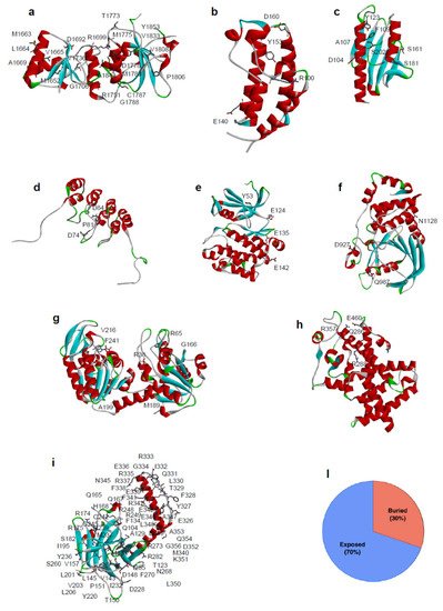
Figure 2. Location of SAVs analyzed in this review and their distribution based on the structural position of the mutated residues. Three-dimensional structure of the proteins analysed in this review are reported. (a) BRCA1 DNA repair associated protein (BRCA1) PDB code: 1JNX, (b) Bromodomain 2(1) (BRD) PDB code: 1X0J, (c) Frataxin (hFXN) PDB code: 1EKG, (d) p16 PDB code: 1DC2, (e) PIM-1 kinase PDB code: 1XWS, (f) Protein tyrosine phosphatase ρ (PTPρ) PDB code: 2OOQ, (g) Phosphoglycerate kinase 1 (PGK1) PDB code: 2XE7, (h) Peroxisome Proliferator Receptor γ (PPARγ) PDB code: 1PRG, (i) Tumor-protein p53 (p53) PDB code: 3Q01. Mutated residues in missense variants are depicted in stick. (l) Distribution of SAVs according to the structural position of the mutated residues for missense variants (30% of the mutation involved buried residues, 70% involved solvent exposed residues).
A further example of the impact of missense mutations on protein stability is represented by the case of hFXN, where 4 out of 8 SAVs show a significant alteration in the thermodynamic parameters (Figure 2c, Supplementary File S1).
In particular, the thermodynamic stability of the hFXN missense variants p.F109L, p.Y123S, p.S161I, and p.S181F is decreased in comparison to that of the wild type, whereas it is unchanged for p.D104G, where a charged polar residue is mutated into a small, uncharged amino acid, for p.S202F, where a polar residue is substituted by a hydrophobic one, and for p.A107V, where the two involved hydrophobic residues differ by their steric hindrance [85].
1.2. Effect on Protein Conformation
Most of the SAVs in our dataset, for which protein conformational changes have been evaluated, e.g., by near-UV Circular Dichroism (CD), or by intrinsic fluorescence changes, show only minor perturbations in the tertiary structure arrangements. Nevertheless, in some SAVs, significant differences in protein conformation were observed, as in the case of p.E135K variant of PIM-1, whose near-UV CD and fluorescence emission spectra dramatically differ from that of the wild-type [86]. The residue E135 is in helix αD and forms a hydrogen bond with Q127, which is likely to be important in stabilizing this helix (Figure 2e and Figure 3a). Notably, a significant reduction in the protein activity was also observed for p.E135K: the mutated protein showed only about 3% of the protein kinase activity of the corresponding wild-type, as well as a decrease in activation energy, which suggests an increase in flexibility with respect to the wild-type counterpart [86].
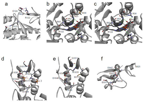
Figure 3. Local environment of SAVs. (a) PIM-1: Detailed view of the local structural environment around the mutated residue E135 [86]; (b,c) PGK1: detail of the 3 phosphoglycerate (3-PG) binding site in the variant p.R38M (b) in comparison with the wild-type (c) [87]; (d,e) BRCA1: Structural rearrangements of p.M1775R variant (d) in comparison with the wild-type, 1 and 2 are two solvent ions (e) [88]; (f) PTPρ: local environment of the mutated residue D927 [77].
The minor conformational changes, observed in SAVs by near-UV CD and fluorescence emission, can also be observed as minimal changes in their 3D structure. The crystal structure of PGK1 p.R38M somatic variant [87] is closely similar to that of the corresponding wild-type and only local differences can be detected. The residue R38 is placed in the N-terminal 3-phosphoglycerate binding domain, where it is important for substrate binding, and its correct positioning is required to react with ADP (Figure 3c).
Moreover, together with residues K215 and K219, R38 is critical for charge balancing of the transition state, directly interacting with the transferring phosphate group in the closed conformation of PGK1. Compared to the wild-type structure, the overall structure of p.R38M is conserved (Figure 2g and Figure 3b,c), with only minor differences between the two: at the level of α-helix 374–382, visible in the p.R38M variant but not in the wild-type, and in the position of the β-phosphate group, which in p.R38M points towards the helix (Figure 3b,c).
Despite the minimal changes in the p.R38M crystal structure, a dramatic effect of mutation on the kinetic parameters of PGK1 was observed; KM increased from 0.40 to 3.15 mM and the turnover number strongly decreased from 89.8 to 7.2 × 10⁻⁶ s−1. This confirms that local and minimal changes in the protein structure, induced by a missense mutation, can lead to major alterations in protein function.
The impact of cancer-related missense mutations on protein structure can be dramatic, as demonstrated by the interesting example of the BRCA1 p.M1775R (Figure 3d). BRCA1 is involved in the regulation of multiple nuclear functions, including transcription, recombination, DNA repair, and checkpoint control, and is frequently mutated in cancer [89]. The p.M1775R variant of the C-terminal domain of BRCA1 (BRCT) cannot interact with histone deacetylases [90], the DNA helicase BACH1 [91], or with the transcriptional co-repressor CtIP [92,93]. The residue p.M1775 is largely buried and its substitution with an arginine residue creates a clustering of three positively charged residues (R1699, R1775 and R1835) (Figure 3d,e). In the wild-type native structure, R1699 participates in the sole conserved salt bridge of the inter-BRCT repeat, formed with a pair of carboxyl-terminal BRCT acidic residues, D1840 and E1836 (Figure 3e). R1835 normally participates in a hydrogen bonding network with Q1811, thereby helping to orient the β1-α1 loop (Figure 3c). In the p.M1775R variant, R1699 retains the salt bridge with D1840 but no longer contacts E1836 and instead coordinates an anion, R1835 rotates away from Q1811 and forms a new salt bridge with E1836 (Figure 3d) [84,88].
1.3. Effect on Protein Interactions
Approximately 60% of disease-associated SAVs show significant perturbations in the protein binding sites, resulting in complete loss of interactions and/or function [94,95,96]. In particular, if the mutated residue is essential in contributing to the interactions with partners [97,98,99,100], the binding affinity, as well as the binding specificity, would be dramatically affected, due to geometrical constraints and/or energetic effects [101,102,103,104]. For example, the deleterious mutations E330K and G352R of SMAD4, clustered near the SMAD4–SMAD3 interaction interface, are associated with juvenile polyposis [105,106]. This observation is in agreement with previous evidence associating the juvenile polyposis with the disruption of the signaling pathway TGFβ/SMAD which includes the interaction of SMAD4–SMAD3 [107,108].
Several SAVs exhibit alterations in their binding properties. An interesting example is represented by the BRDs, small helical interaction modules that specifically recognize acetylation sites in proteins. BRD2(1) (Figure 2b) and BRD3(2) SAVs show significant differences in their binding to two inhibitors of pharmacological interest, PFI-1 and JQ1, that may be related to the location of the missense mutations in proximity of a region important for the binding to acetylated peptides [109].
1.4. Effect on Protein Catalytic Activity
In the human population, 25% of the known SAVs show a significant modification of their biological function [76]. This percentage is mostly covered by mutations that occur in the active sites of enzymes or in the binding pockets of receptors [110,111]. Biochemical reactions are very sensitive to the precise geometry of the active sites [112,113,114]. Enzyme catalysis, however, does not depend just on a restricted number of crucial residues in the catalytic pocket, but also on several surrounding residues, important for ensuring the proper positioning of the substrates and cofactors into the active site. Therefore, mutations that occur on the residues located in the neighborhood of the active site, although not directly involved in the catalytic event, may also influence the enzyme activity [112,113], as in the case of PGK1 SAVs, discussed in Section 3.2 (Figure 3b). An interesting example of changes in enzyme tyrosine phosphatase activity, due to the presence of missense mutations, is represented by the case of PTPρ (Figure 2f), that belongs to the classical receptor type IIB family of protein tyrosine phosphatase and may act as a tumor suppressor [115]. Among the PTPρ SAVs identified in human cancer tissues, the missense variant p.D927G is almost completely inactive at 37°C [77]. This mutation involves a solvent exposed residue, distant from the catalytic site, and placed in a 4-residues turn between two coils, that connects different secondary structure regions through hydrogen bonds with three residues (D947, K930, and E931) (Figure 3f). The highly destabilizing D927G mutation may presumably alter the main chain flexibility, leading to local disorder, and thus affecting the stabilizing hydrogen bonds of residues in its proximity [77]. This SAV is an interesting example of the cumulative effect of a missense mutation on thermodynamic stability and function.
2. Computational Analysis of Protein Variants in Cancer-Related Genes
The large amount of protein variants collected in public databases and the limitations in the experimental methods stimulated the development of several tools for predicting their impact on protein stability and their pathogenic effect. Accordingly, early developed tools focus on the prediction of protein stability change by estimating the variation of free energy change (ΔΔGf) resulting from an amino acid substitution [116,117]. The majority of methods, which have been trained on ProTherm database [118] or on manually collected datasets [26], predict either the value or the sign (positive/negative) of the ΔΔGf. More recently, once large databases collecting pathogenic variants were made available, many binary classifiers have been implemented for predicting the impact of genetic variants on human health [119,120,121]. All available methods for predicting the impact of variants on protein stability or on protein pathogenicity rely on the various features extracted from protein sequence, structure, and evolutionary information. State-of-the-art methods of both types are currently used for protein engineering and for variant interpretation. In this section, we analyze the effect of the protein variants using computational approaches for predicting protein stability changes and pathogenicity, with the aim of estimating the role of protein stability on cancer mechanisms and the reliability of computational tools on this specific task.
2.1. Collection of the Protein Variant Datasets
In this work, we analyze a set of 164 missense variants from 11 proteins to understand the contribution of protein stability on the insurgence and progression of cancer (Table S1). Among the 11 proteins, 5 of them are mainly involved in regulation activities (BRD2, BRD3, BRD4, p16, and PPARγ), 4 have catalytic activities (PIM1, PGK1, FXN, and PTPρ) while the remaining 2 (p53 and BRCA1) are involved in many biological processes. The set collects all protein variants, for which the folding ΔΔG value was experimentally determined and whose genes are reported in the COSMIC database, either as Tier 1 genes, or with putative cancer-driving evidence. The folding ΔΔGf is calculated as the difference between the folding ΔG of the mutant and wild-type proteins (ΔΔGf = ΔGfmut − ΔGfwt), i.e., it is positive for destabilizing variants. When available, the variation of the melting temperature (ΔTm = Tmmut − Tmwt) was also collected. The distributions of the ΔΔGf and ΔTm values are plotted in Figure 4a. The protein mutants are mapped on unique protein structures except in the case of p53, for which the DNA binding and oligomerization domains are considered separately. A subset of 97 variants from 9 proteins is obtained by matching our dataset with the data collected by the Cancer Mutation Census (CMC) project. This subset is composed of 24 putative cancer-driving variants annotated as “Tier 1–3” and 63 putative benign variants annotated as “Other”.
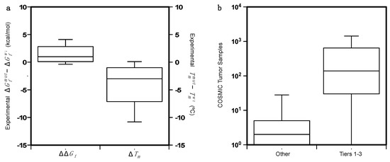
Figure 4. (a) Distributions of the of ΔΔGf and ΔTm on the dataset of 164 protein variants. ΔTm is available only for 73 of them. (b) Comparison of the distributions of the COSMIC tumor samples for the putative cancer-driving variants (Tiers 1–3) and the benign variants (Others) annotated by the Cancer Mutation Census project.
In Figure 4b we compared the distribution of the COSMIC tumor samples in which the putative cancer-driving variants (PCVs) and putative benign variants were detected. The somatic variants annotated by the CMC project are found in different tumor tissues. In particular, the hotspot mutants in the p53 DNA-binding region are detected in tumors from more than 30 tissues.
2.2. Analysis of the Protein Variants
In this review we verified the possibility of using the available methods for predicting the impact of missense variants to identify key functional residues of the protein. We first evaluated the performance of a state-of-the-art method (FoldX [27]) in the prediction of ΔΔGf resulting from an amino acid substitution. In the second step of the analysis, we predicted the pathogenicity of the selected variants to identify putative cancer-driving variants. For this task we used Meta-SNP [28], a meta prediction algorithm combining the output of 4 methods, namely PhD-SNP [122], PANTHER [123], SIFT [124], and SNAP [125]. The Meta-SNP output is considered as a proxy for predicting PCVs as reported in the Cancer Mutation Census (https://cancer.sanger.ac.uk/cmc (accessed on 1 May 2021)). For optimizing the prediction process on our set of cancer-associated genes we performed a 5-fold cross-validation procedure to select the best classification threshold. For a better characterization of the results, we also evaluated the importance of protein structure and evolutionary information in the detection of putative cancer-driving variants.
2.3. Predicting the Folding Free Energy Change of the Protein Variants
For each mutant in our dataset, we predicted the variation of the folding free energy (ΔΔGf) using FoldX, which is one of the most accurate methods for such a task [79]. For each mutant, we averaged the FoldX predictions on 10 models of the mutated structure. We then compared the predicted and the experimental ΔΔGf values and calculated the performance on the set of variants, either grouped by proteins or on the whole set. In particular, we calculated three types of correlation (Pearson, Spermann, Kendall-Tau), and two error estimates, the Root Mean Square Error (RMSE) and the Mean Absolute Error (MAE). The results in Table S2 show that, on the whole set of 164 variants, FoldX achieves a Pearson correlation coefficient (rP) of 0.50 and a RMSE of 2.1 kcal/mol. This result can be improved by removing the variant p.G1788V of BRCA1 from the dataset. For that variant, FoldX predicts a ΔΔGf of 15.2 kcal/mol, which is much higher than all other predicted values. Such a large predicted ΔΔG value is likely due to a limitation of FoldX, which in this case fails to identify a stable conformation of the protein mutant. After removing p.G1788V from the dataset, the rP increased to 0.56 and the RMSE decreased to 1.8 kcal/mol. On average we observed that the predicted ΔΔG values returned by FoldX tend to be larger than the experimental values. This behavior is probably due to the implementation of the FoldX algorithm which predicts the structure of the mutant protein only considering different rotamers of the amino acid side chains. Such a process might limit the ability of the tool to identify more stable conformations that could be obtained through the rearrangement of the backbone.
Further analysis was performed after grouping the variants by proteins and calculating the performance on the resulting protein subsets. By doing so, we observed for some proteins (both domains of p53, hFXN, PGK1, and PTPρ) a rP > 0.58. For other proteins (BRDs, PIM-1, and p16) with a smaller number of mutants (≤10), we observed lower or negative correlation coefficients. The scatter plots, showing the correlation between predicted and experimental ΔΔGf values for the whole set of proteins, or for the proteins with the highest number of mutants (p53 and BRCA1), are shown in Figure 5. Another interesting analysis consists in the prediction of highly destabilizing variants (ΔΔGf > 2 kcal/mol). In this case, we have used FoldX as a binary classifier, optimizing a threshold on its output.
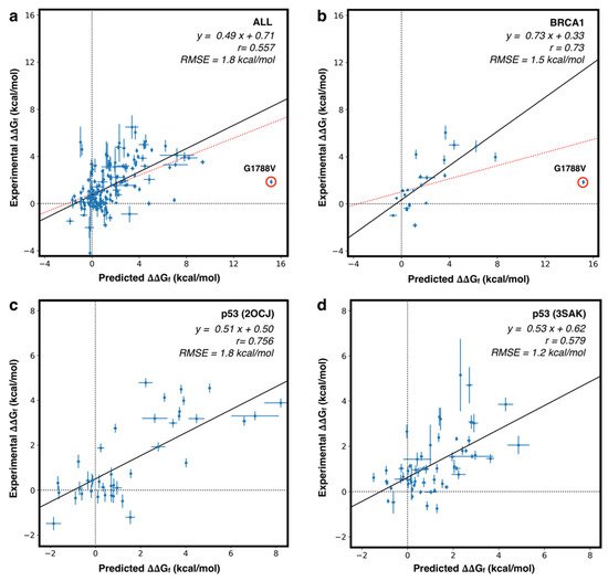
Figure 5. Scatter plot for predicted vs experimental ΔΔGf values. (a) fitting on the whole set of 164 variants (red) and after removing the outlier BRCA1 p.G1788V (black). (b) Similar analysis performed on the whole set of variants in BRCA1 (red) and after removing BRCA1 p.G1788V variant (black). (c,d) fitting on the subset of variants in p53 core (2OCJ) and oligomeric (3SAK) domains, respectively. r: Pearson correlation coefficient. RMSE: Root Mean Square Error.
The optimization procedure, based on balancing the true positive and true negative rates, shows that FoldX can achieve an overall accuracy of 77% and a Matthews Correlation Coefficient (MCC) of 0.55 when a prediction threshold of ~1.2 kcal/mol is considered for the whole set of 164 variants. This method shows a good performance also when considering protein-specific thresholds. Indeed, for the subset of proteins with the highest number of mutants (p53 and BRCA1), the performance in the classification task reached MCC = 0.78 and AUC (Area Under the ROC curve) = 0.95 for the DNA binding domain of p53, or MCC = 0.67 and AUC = 0.90 for BRCA1. All performance measures in the classification task are summarized in Table S3.
In general, our analysis confirms that, on average, the predicted and experimental ΔΔGf correlate well, and that the FoldX prediction can be used to estimate the impact of mutations of protein stability, in spite of the fact that the prediction error still remains ~2.0 kcal/mol. To partially address this limitation, the methods for ΔΔGf prediction can be used as binary classifiers to detect highly destabilizing protein variants.
2.4. Predicting the Pathogenicity of Protein Variants
In the last decade, several methods have been developed for predicting the pathogenicity of variants. In general, those approaches are binary classifiers, based on the analysis of evolutionary conservation. The idea behind these tools is based on the observation that mutations occurring in highly conserved regions of the protein are more likely to be pathogenic than mutations in variable regions. In the case of cancer-associated variants, the validation of the predictive methods is a difficult task due to the lack of curated sets of annotated variants. To address this issue, the COSMIC curators are annotating the somatic mutations in the Cancer Mutation Census (CMC) dataset [19]. Currently, the CMC contains ~3 million missense variants, only ~0.1% of which were curated. Using such annotation, we analyzed the prediction of Meta-SNP, an algorithm combining the output of 4 methods, on our dataset. Initially, we analyzed the relationship between the experimental ΔΔGf and the variant pathogenicity score returned by Meta-SNP, to test its performance in the detection of highly destabilizing variants (ΔΔGf > 2 kcal/mol). Setting the optimized classification threshold to 0.66, we found that Meta-SNP reaches an accuracy of 73% and a Pearson correlation coefficient of 0.40 in the classification of highly destabilizing variants. We also estimated the performance of Meta-SNP in the prediction of putative cancer-driving variants (PCVs), assuming that missense variants, annotated as “Other” in the CMC database, can be classified as benign and variants in CMC annotated as classes 1–3 (Tier 1–3) can be considered putative cancer-driving variants (PCVs). For a more stringent test we calculated the performance of Meta-SNP by removing from the dataset 15 mutations used for the training of the method. Our results show that, for the subset of 82 variants annotated in CMC, by using a classification threshold of 0.71, Meta-SNP is able to predict PCVs with 77% accuracy and a Matthews correlation coefficient of 0.37.
The high fraction of false positives in the prediction of highly destabilizing variants may indicate the presence of pathogenicity mechanisms alternative to the loss of stability, while the high rate of false positives in the prediction of PCVs can be due to incorrect and/or incomplete protein variants annotation.
Although the Meta-SNP predictions result in a high fraction of false positive, the PCVs, annotated with 1 to 3 in the CMC database, are enriched in the variants with folding ΔΔGf > 2 kcal/mol with respect to the subset of CMC variant annotated as “Other”. Indeed, the relative p-value calculated by the Fisher test is <0.03.
Furthermore, the comparison of the distributions of the Meta-SNP output for Tier 1–3 and “Other” variants reveals a significant difference. The average values of the distributions of Meta-SNP outputs for Tier 1–3 and “Other” variants are 0.71 and 0.47, respectively. This difference is statistically significant, corresponding to a Kolmogorov-Smirnov p-value < 10−4.
Finally, we also tested the performance of FoldX in predicting PCVs. Our analysis revealed that, selecting a predicted ΔΔGf threshold of 2.7 kcal/mol, FoldX is able to identify Tier 1–3 variants with 73% overall accuracy and a Matthews correlation coefficient of 0.33. The comparison of the results shows that a predictor of putative pathogenic variants (Meta-SNP) is performing better than a method designed to predict folding ΔΔGf (FoldX) in the detection of PCVs.
2.5. Analysis of the Prediction on the Basis of the Amino Acid Accessibility and Conservation
In the previous sections, we have shown that protein stability of cancer-related genes can be predicted with a good level of confidence using dedicated computational tools like FoldX. We have also observed that the pathogenicity score, calculated through a consensus method, correlates with protein stability data and with phenotypic data. Nevertheless, the prediction of PCVs, starting from protein stability predictions, is a more complex task. To this end, more experimental data on the stability of cancer proteins and their variants, and a higher level of curation of the existing databases on cancer protein variants would be needed. As an in-silico alternative for estimating the impact of protein variants on the stability and phenotypic levels, we used Meta-SNP, which is one of the state-of-the-art methods that best predict the protein variant pathogenic potential. To better analyze the results obtained by Meta-SNP, we calculated the distributions of solvent accessibility and conservation scores of the wild-type residues for the subset of highly destabilizing and PCVs.
In detail, for each mutated site we calculated the relative solvent accessibility (RSA) of the mutated residues and the frequency of the wild-type residue in the multiple sequence alignment (fWT) of possible homologs of the mutated protein.
As described in supplementary materials, the RSA was calculated by normalizing the solvent accessibility calculated with the DSSP program [126] and the fWT was returned as part of the output of the Meta-SNP server (http://snps.biofold.org/meta-snp, accessed on 1 May 2021). In the first part of our analysis, we compared the RSA values for the subset of highly destabilizing variants (ΔΔG > 2.0 kcal/mol) and the remaining ones, showing that for RSA ≤ 0.2 there is little overlap between the two distributions (Figure 6a). In the same range of RSA (Figure 6b), the PCVs (Tiers 1–3) can be easily discriminated from benign ones (“Other”). In both cases, using the Kolmogorov-Smirnov test to estimate the statistical difference between the two subsets in Figs. 6a and 6b, we obtained p-values < 10−3. In particular, Figure 6b shows that the majority of PCVs (~58%) are occurring in buried regions (RSA ≤ 0.2), while ~75% of putative benign variants are in exposed regions (RSA > 0.2). The fraction of PCVs in exposed regions, which we found in our dataset, is higher than the value reported for pathogenic variants [63], nevertheless, due to the reduced size of our dataset, such a difference is not statistically significant.
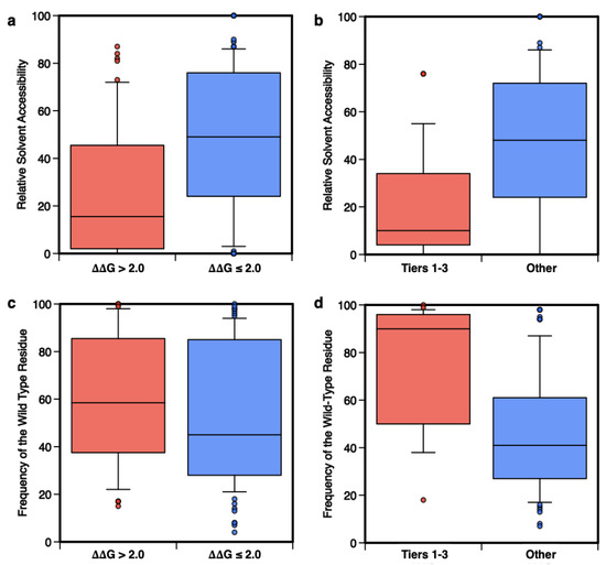
Figure 6. Distributions of the Relative Solvent Accessibility (RSA) and frequency of the wild-type residue (fwt) in the multiple sequences of homolog proteins. The distributions of RSA and fwt calculated for the subsets of 53 highly destabilizing variants (ΔΔGf > 2.0 kcal/mol) compared to the remaining 111 variants (ΔΔGf ≤ 2.0 kcal/mol) are shown in panels (a,c). In panels (b,d) the same distributions are plotted for the subsets of 24 putative cancer-driving (Tier 1–3) or 73 benign (‘Other’) variants.
In the second part of this analysis, different results are observed when the distributions of fWT are compared. Figure 6c shows that conservation is not a strong feature for the classification of highly destabilizing variants, while it is essential for the prediction of PCVs. Indeed, for fWT > 50% the distributions of Tier 1–3 and “Other” variants have little overlap (Figure 6d). The comparison between the results in Figure 6c,d indicates that destabilization and conservation may indeed serve the pathogenicity prediction task as reciprocally integrating features [25].
A further interesting analysis can be performed by considering the distribution in two dimensions of the RSA and fWT together for Tiers 1–3 and “Other” variants. In Figure 7a we observed an enrichment for Tiers 1–3 variants in the buried (RSA < 20%) and conserved residues (fWT > 50%), with a corresponding p-value of 3 × 10⁻⁶, obtained by considering a binomial distribution with a success probability of 0.247. On the opposite side of the plot (RSA ≥ 20% and fWT ≤ 50%), we observed a depletion of PCVs (p-value = 0.02). Finally, we performed a similar analysis by combining the experimental ΔΔGf with the Meta-SNP predictions (Figure 7b).
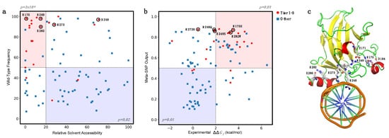
Figure 7. Enrichment and depletion of putative cancer-driving variants (Tier 1–3) in different subgroups. (a) Enrichment of Tier 1–3 variants in mutated sites with Relative Solvent Accessibility ≤20% and frequency of the wild-type residue > 50% (light red). (b) Enrichment of Tier 1–3 variants in the subset of mutants with experimental ΔΔGf > 2.0 kcal/mol and Meta-SNP output >0.5 (light red). In both cases, the opposite regions (light blue) are depleted of Tier 1–3 variants. In (a,b), the hotspot mutants R175, R248, R249, R273, and R282 are highlighted with black circles. (c) Hotspot sites in the p53 structure in interaction with DNA (PDB:1TUP). Residues R248 and R273 interact with DNA. Residues R175, R249, and R282 are likely to stabilize the protein structure by forming salt bridge interactions with D162, E171, and E286, respectively.
If we considered the subset of highly destabilizing (ΔΔGf > 2.0 kcal/mol) and predicted pathogenic (Meta-SNP output > 0.5) variants, we found an enrichment in Tier 1–3 variants with corresponding p-value of 0.01. On the opposite side of the plot, we observed a depletion of Tier 1–3 variants, again with a p-value of 0.01.
These observations confirm the hypothesis that relative solvent accessibility and amino acid conservation are important features for predicting the impact of amino acid substitution in terms of protein stability and pathogenicity. Furthermore, the combination of the experimental ΔΔGf and the predicted pathogenicity of variants allows to select a subset of variants with a significantly high probability of having a deleterious phenotypic effect.
In particular, focusing on a subset of five hotspot sites of p53 [127,128], we observed that R248 and R273 are directly interacting with the DNA, in agreement with their high RSA, while R175, R249, and R282 (low RSA) are surrounding the DNA binding site (Figure 7c). These structural aspects, combined with our predictions, support the hypothesis that the p.R248Q and p.R273H variants (with high pathogenicity score but low ΔΔGf) have a direct impact on the protein function of DNA-interaction, while p.R175H and p.R282W (with both high pathogenicity score and high ΔΔGf) destabilize the p53 structure. An intermediate case is p.R249S, which shows a variation of folding free energy of ~2 kcal/mol and a low RSA. Similar to R175 and R282, the presence of an oppositely charged residue (E171) in the proximity of R249 suggests that a mutation in this site can indeed reduce the stability of p53, due to a missing salt bridge interaction. Although a significant difference between predicted and experimental ΔΔGf values (RMSE = 3.2 kcal/mol) is observed for the five hotspots, similar results are obtained when combining the Meta-SNP output with the predicted ΔΔGf (Figure S1). Our analysis can be compared with the experimental data on DNA-binding affinity of the p53 mutants [82]. The data show that among the five hotspots cancer mutants shown in Figure 7, the three of them with low impact on p53 stability (p.R248Q, p.R249S, and p.R273H with ΔΔGf ≤ 2.0 kcal/mol) had no detectable binding affinity with the gadd45 promoter DNA (0% with respect to the wild type). This observation supports the hypothesis that protein–DNA interactions may play an important role in the cancer-inducing mechanism of the mutated p53. By analogy, a similar case of compromised protein–DNA or protein–protein interactions might turn out to hold for other cancer-associated mutants, which might not be in the ‘highly destabilizing’ category. The above observation is also in agreement with the possible roles hotspots cancer p53 mutants are considered to play as gain-of-function effectors [127,128], not only for the ‘contact’ mutants p.R248Q and p.R273H, but also for the ‘conformational’ mutants p.R175H, p.R249S, and p.R282W, since an altered p53 binding energy landscape can shift the mutated cells to different functionalities. Furthermore, the data shown in Figure 7 are consistent with the fact that also destabilizing variants can have gain-of-function characteristics, possibly through altered protein–protein interactions [56].
This entry is adapted from the peer-reviewed paper 10.3390/ijms22115416
This entry is offline, you can click here to edit this entry!