Your browser does not fully support modern features. Please upgrade for a smoother experience.
Please note this is an old version of this entry, which may differ significantly from the current revision.
Subjects:
Materials Science, Biomaterials
Cellulose is the most common biopolymer and widely used in our daily life. Due to its unique properties and biodegradability, it has been attracting increased attention in the recent years and various new applications of cellulose and its derivatives are constantly being found. The development of new materials with improved properties, however, is not always an easy task, and theoretical models and computer simulations can often help in this process.
- cellulose
- coarse-grained
- molecular simulations
1. Cellulose
Cellulose is among the most abundant biopolymers on Earth, and it roughly comprises around 30% of all vascular plants [1]. Cellulose provides mechanical stability and durability to plants. In one or another form, cellulose has been used by humanity for thousands of years. In the recent decades, it has attracted a renewed interest in the scientific community due to its widespread abundance and excellent mechanical properties, which could be further altered by chemical modifications [2][3].
Cellulose is a polysaccharide made of α-D-Glucopyranose units (AGU) linked by β(1→4) glucosidic bonds. The polymer chains consist of hundreds to thousands of glucose units depending on the cellulose source—plants or bacteria. The individual cellulose chains are arranged in a precise crystallographic pattern denoted as cellulose I, where two naturally occurring allomorphs exist—cellulose Iα and Iβ [4]. Up to 36 cellulose chains can form the so-called primitive fibril (cellulose nanofibril, or CNF) in plants, and several such fibrils can form micro- and macrofibrils. Finally, bundles of many macrofibrils form cellulose fibers [5][6][7]. However, during the industrial processing, cellulose fibers can be broken down to the primitive fibrils and moreover only the crystalline part of the fibrils can be extracted after acid treatment [8]. These crystals are often referred to as cellulose nanocrystals (CNCs), and have dimensions most often of hundreds of nanometers in length and around 3–5 nm in width [9]. CNCs have high aspect ratio and excellent mechanical properties. Therefore, CNCs were utilized for many applications in various fields ranging from medicine [10] to environmental science [11][12] and energy storage [13], to name a few. However, one particular characteristic of cellulose can be even as important as its excellent mechanical properties and this is that cellulose is a biobased, and thus biodegradable material. This makes cellulose a promising sustainable material with many possible applications.
A substantial part of the scientific knowledge about cellulose was obtained empirically. During past decades, theoretical modelling, molecular simulations and ab initio calculations became the valuable and often essential tools providing a fundamental insight into materials’ properties. Cellulose has also been studied through the years using theoretical and simulation approaches. However, the modelling of experimentally relevant systems can be hindered by the time and spatial scales which are too large and thus, can be hardly accessible by standard all atomistic molecular simulations. Therefore, many researchers have developed and used coarse-grained (CG) simulations to model cellulose systems on large spatio-temporal scales. In the CG simulations, several atoms are combined in so-called beads, which makes it possible to model larger systems on longer time scales. Many different CG models of polysaccharides were developed during the last few decades, and they will be presented in this review. There have been an increased number of newly developed CG models in the recent years, which to some extent correlates with the renewed interest to cellulose from the wider scientific community.
2. Coarse-Grained Modelling
Coarse-grained (CG) models describe the atomistic structure (fine-grained) of molecules and materials with a reduced representation. The atoms representing a given functional group or a molecule are grouped (mapped) into a single particle, often referred to as the “interaction site”, “bead”, “particle”, or “superatom”. Thus, the number of particles required to describe a given molecular structure are smaller compared to all-atom models. In this way, the simulations can be significantly accelerated and therefore it is possible to reach longer simulation times and bigger spatial domains, compared to the corresponding all-atom simulations. It is noteworthy that a particular choice of the beads in the CG mapping is not unique, and is often guided by the experience and chemical intuition. Therefore, for a particular molecule, many different mapping schemes may exist. The mapping of the atoms into one bead is typically carried out with the help of a mapping operator (MI) that determines the coordinates of the I-th CG particle (RI) from a linear combination of the Cartesian coordinates (ri) of the atoms belonging to a particular group in the atomistic representation.
RI=MI(r)=∑icIiri
The beads’ positions determined in this way are usually chosen as the center of mass or center of geometry (geometrical center) of the particular group of atoms from the atomistic representation. With the advancement of computational techniques and machine learning, new ways to construct and map the atoms into the CG bead have been developed, which might help to remove the human bias and potentially develop better CG models [14][15][16].
After mapping the atomistic structure into a desired CG representation, one should assign the potential functions determining the bonded and non-bonded interactions of the model, and consequently validate these functions against atomistic simulation or experimental results. Using atomistic simulations to develop the CG potentials is known as a bottom–up approach, while using experimental data to fit the potential is referred to as a top–bottom approach. There are several techniques that are often used to fit a CG potential based on the all-atom simulations, including Boltzmann inversion, inverse Monte Carlo [17][18], relative entropy [19], force matching (multiscale coarse-graining) [20][21], and the realistic extension algorithm via covariance hessian (REACH) [22]. The purpose of this review, however, is not to provide detailed descriptions of these methods, and we therefore can refer an interested reader to other review papers describing these methods in more detail [23][24][25].
Undoubtedly, the most widely used CG force field nowadays is the Martini force field [26]. This force field was parameterized against experimental partition, vaporization and hydration free energies and therefore is considered as a top–down approach. Martini was originally developed for biomolecular systems, such as lipid membranes. However, since then it has been used to model different material systems and many CG molecule models have been built with Martini, including cellulose and other polysaccharides [27][28][29][30].
3. Coarse-Grained Models of Carbohydrates
Different CG models for mono- and polysaccharides have been developed through the years [27][28][29][30][31][32][33][34][35][36][37][38][39][40][41][42][43][44][45][46][47][48][49][50][51][52][53][54][55][56][57][58]. Often, these CG models possess different mapping of the anhydroglucose units (AGUs), thus providing a different level of detail of the models. Figure 1 presents the most commonly used mapping schemes (found in more than one publication) for polysaccharides. In many studies, each AGU has been represented by three CG beads [27][28][29][31][35][36][38][39][42][43][57]. Two widely used mapping schemes with three CG beads are illustrated in Figure 1a,b.
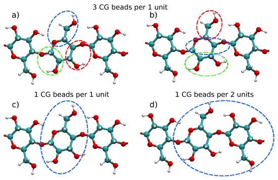
Figure 1. Different coarse-grained mapping schemes for polysaccharides and cellulose with mapping of (a) 3-to-1 (coarse-grained (CG) beads per 1 glucose unit), (b) Martini force field 3-to-1 (CG beads per 1 glucose unit), (c) 1 CG bead per 1 glucose unit and (d) 1 CG bead for 2 glucose units.
Molinero and Goddard [31] pioneered the CG modeling of polysaccharides with their M3B model, which uses a mapping scheme presented in Figure 1a. Originally, the M3B model was derived for α(1→4) D-glucan oligosaccharides and its extension to other linkage types, such as α(1→6) and β(1→4) glucans, was discussed as well. This model used Boltzmann inversion to parameterize the bonded interactions and a Monte Carlo simulated annealing to obtain the non-bonded parameters, which were modeled by the Morse potential. The same mapping as in the M3B model was subsequently adopted in several other studies [35][36][38][39][57]. Although in these studies, the mapping scheme is similar, the potential functions used to represent the interactions (bonded and non-bonded) are different. Hence, the models are effectively different from each other. Liu et al. [35] used a multiscale coarse-graining to derive parameters for α-D-glucopyranose in an aqueous solution. A CG model of cellulose Iβ microfibril hydrophobic surface was developed using the same three bead mapping scheme by Bu et al. [36]. This model reproduced the crystal structure of the Iβ fibril well and modeled its interactions with the Trichoderma reesei cellobiohydrolase I enzyme, which is used in cellulose enzymatic degradation. Two more models utilizing the CG scheme depicted on Figure 1a were developed for β-D-glucose, cellobiose and cellotetraose [38][39]. Markutsya et al. in the same paper [39] also presented a six particles model, showing that it provides a higher level of structural accuracy than the three beads model for glucose. This is not surprising because of the usage of twice the number of beads for glucose, which also increases the computational cost of the CG model. However, an interesting observation is that placing the CG beads either at the center of mass (COM) or at the center of geometry (COG) of the respective groups of atoms leads to a difference in the radial distribution functions (RDFs). In the three beads model, the usage of COM provides better results, while in the six beads model the COG mapping yields more accurate RDFs. In a follow-up study, an evaluation of different CG mapping schemes in a cellulose microfiber was performed for mapping of one, two, three or four CG beads per glucose unit [43]. According to this study the one- and two-bead models are suitable for simulating long time-scales properties of microfibers, such as transitions from crystal to amorphous structures. The more detailed models (three and four beads) provide a better level of detail and are able to reproduce the conformational changes in the glucose residues.
The Martini models of mono- and oligosaccharides adopt the mapping schemes presented in Figure 1a,b, respectively [27]. It was shown that with these models, a broad palette of polysaccharides can be simulated and their structural and dynamical properties can be well described, although hydrogen bonds are in principle neglected. Wohlert and Berglund [28] adopted the Martini model with three bead mapping (Figure 1b) to construct a CG model of a cellulose Iβ crystal. The crystalline microfiber model for cellulose was further utilized and extended showing the transformation of cellulose Iβ to IIII allomorph [29]. A recent noteworthy application of the Martini force field is the extension to N-glycans by Shivgan et al. [30]. The authors explored various branching patterns in N-glycans and they used the CG mapping for the glucose monomer unit presented in Figure 1b.
Although the three bead models described above were successfully used to model cellulose nanocrystals and fibers, they still can be computationally expensive for long fibers typically studied experimentally and found in nature. Therefore, many simulations utilize even more coarse-grained representation for cellulose fibers, such as mapping one or two glucose units (Figure 1c,d) into a single CG bead [33][37][40][44][46][47][48][50][51][52][53][59]. The positions of the CG beads are located either at the center of the glucose unit or at the O4 atom, i.e., at the center of the glucosidic bond. With careful parameterization against atomistic molecular dynamics (MD) (mostly utilizing the Boltzmann inversion method), all of these single bead models reproduce the crystallographic structures of the Iα or Iβ cellulose allomorphs very well. Recently, Shishehbor and Zavattieri [53] developed a coarse-grained model that uses one CG bead for two glucose units (Figure 1d). In their model, the bonded interactions are represented by Morse potential, which enables bond breaking and allows one to describe cellulose fibril dissociation under mechanical stress. The model is thoroughly validated against various mechanical and interfacial properties.
Up to now, we described the most commonly used mapping schemes for the CG modeling of polysaccharides, with a main focus on cellulose models. However, in the recent years, several standalone models with different mapping philosophies than the ones described above, have been developed [41][54][55][56][60][61]. Wu et al. [56] developed a CG model similar to the one that they used earlier for α-1,3-glucans, [62] to the directional hydrogen bonding of cellulose chains. This model, depicted in Figure 2a, has one backbone bead (BB) representing the pyranose ring, one “satellite” bead (SB) for the hydroxymethyl group and a linker bead used as a connection point for some of the bonded interactions in model. The hydrogen bonds are accounted for by the so-called “hydrogen bonding beads” (DCX).
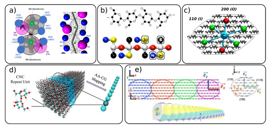
Figure 2. Mapping schemes for cellulose with different degree of mapping where one glucose unit is mapped with (a,b) several beads or (c–e) whole section of the cellulose fibril is mapped with 1 CG bead. Figure adapted with permissions from references (a) [56], 2020, American Chemical Society (ACS) (b) [41], 2012, American Chemical Society (ACS) (c) [54] 2020 Springer, (d) [60] 2020 Elsevier and (e) [55] 2020, American Chemical Society (ACS). CNC: cellulose nanocrystal, AA: all-atom.
Bellesia et al. [41] developed a CG model of cellulose to study the conversion of cellulose Iβ to IIII. The model, shown on Figure 2b, is constructed from five beads and successfully predicts the thermodynamical properties and structures of the concerned cellulose allomorphs in the implicit solvent using Langevin dynamics.
Recently, several CG models for cellulose nanofibers were developed where the whole part of the nanofiber including many glucose units are mapped into one CG bead [54][55][60]. The supra coarse-grained (sCG) model [54] (Figure 2c) uses seven beads to map the entire cross-section of the 36 chain-model of the cellulose nanofiber. Each surface bead represents 20 glucose units (five units across nanofiber and four units along the axial direction) and two types of surface beads were designed to reproduce surfaces with different water affinity (hydrophilic and hydrophobic). The central beads describe 24 glucose units and act as the backbone of the nanofiber, being mainly responsible for the mechanical properties (elastic modulus) of the structure. Each central bead is connected to the neighboring central beads and to six surface beads by the harmonic bonds. There are no CG bonds between the surface beads. The bonded interactions of the sCG model were parameterized with the force matching procedure and the non-bonded interactions against the atomistic potential of mean forces. The model was used together with Langevin dynamics; thus, no explicit water molecules are needed, which allows one to study a large system on the scale of hundreds of nanometers in a microsecond range.
The “bead-spring” CNC mesoscopic model [60][61] developed by Qin and co-workers [61] and later utilized by Li et al. [60] (Figure 2d) maps the whole cross-section of 36 chains with three repeated units into one CG bead. This model was used to investigate the mechanical properties of CNC nanopaper and CNC bulk materials forming a porous network structure.
Another mesoscopic model for CNC was developed by Rolland et al. [55]. This model is an extension of the Kern–Frenkel patchy particle model [63] where one CG bead represents a cross-section of 36 chain-model of a CNC with eight glucose units along the axial direction (Figure 2e). Thus, one CG bead contains around 6000 atoms. The bead particles have an aspherical shape, and each bead is decorated with anisotropic patches, which are different depending on the surface type, with 100, 110, 1–10 surfaces being considered. The patches describe the non-bonded interactions between the CNC particles. The bonded and non-bonded interactions in the model were parameterized against atomistic MD simulations, including the bond and angle distributions and potentials of mean forces, respectively. It should be noted that the patchy particle models have great potential for future use, since one can create different types of patches and interactions, allowing for large flexibility and fine tuning of the interactions.
A scalable CG scheme was recently used to model CNC where the mapping and interaction potentials are scaled on three different levels (Level 1–3) and are based on atomistic simulations [59]. The different levels represent 1 glucose unit (Level–1), six Level-1 beads are mapped into one Level-2 bead and seven Level-2 chains form one Level-3 bead.
Shishehbor et al. [64] presented a continuum-based approach to model cellulose nanocrystals, and although this model is not strictly a particle-based coarse-grained one, it is also worth to be mentioned in this review. The individual chains in the CNC are modeled as elastic beams passing through the center of mass of the CNC. The elastic characteristics of the beams are obtained from atomistic simulations of cellulose chains, and each beam element represents one or more glucose monomers.
4. Applications of Cellulose CG Models
In this section, we discuss different applications of the CG cellulose models presented in the previous section. Many of the mentioned studies extensively discussed the performance of the CG models against atomistic simulation, which is important for the validation of the models. In the present section, we focus on the results of the CG simulations for cellulose nanocrystals and fibers towards describing specific cellulose material properties, and we therefore will not discuss results describing the validation of the CG simulations.
4.1. Mechanical Properties
Mechanical properties on a single fibril level [40][51][54][64], fibrils bundles [52][53] and cellulose networks [53][54][60][61] have been widely investigated by coarse-grained simulations. The Young’s modulus in the longitudinal (EY) and transverse (ET) directions on a single fibril level were calculated with the REACH [40] CG model (Figure 3a) for cellulose Iβ and by Poma et al. [51] for both cellulose Iβ and cellulose Iα. EY was estimated to be between 110 and 162 GPa, which falls in the somewhat wide experimental range of 93–220 GPa, as reported in the work of Glass et al. [40] The transverse modulus calculated in these works [40][51] are found to be in the range of 7–41 GPa. In the continuum-based approach of Shishehbor et al. [64] they obtained values for EY = 147 GPa and ET = 6.5 and 19 GPa. Figure 3a also shows the variation of EY with the temperature obtained with the REACH model, which shows a linear decrease with increasing T. All of the CG models discussed above are based on the 36 chain CNC model, and they show consistent results comparable with the experimental ones, although the CG models are quite different and parameterized using various techniques.
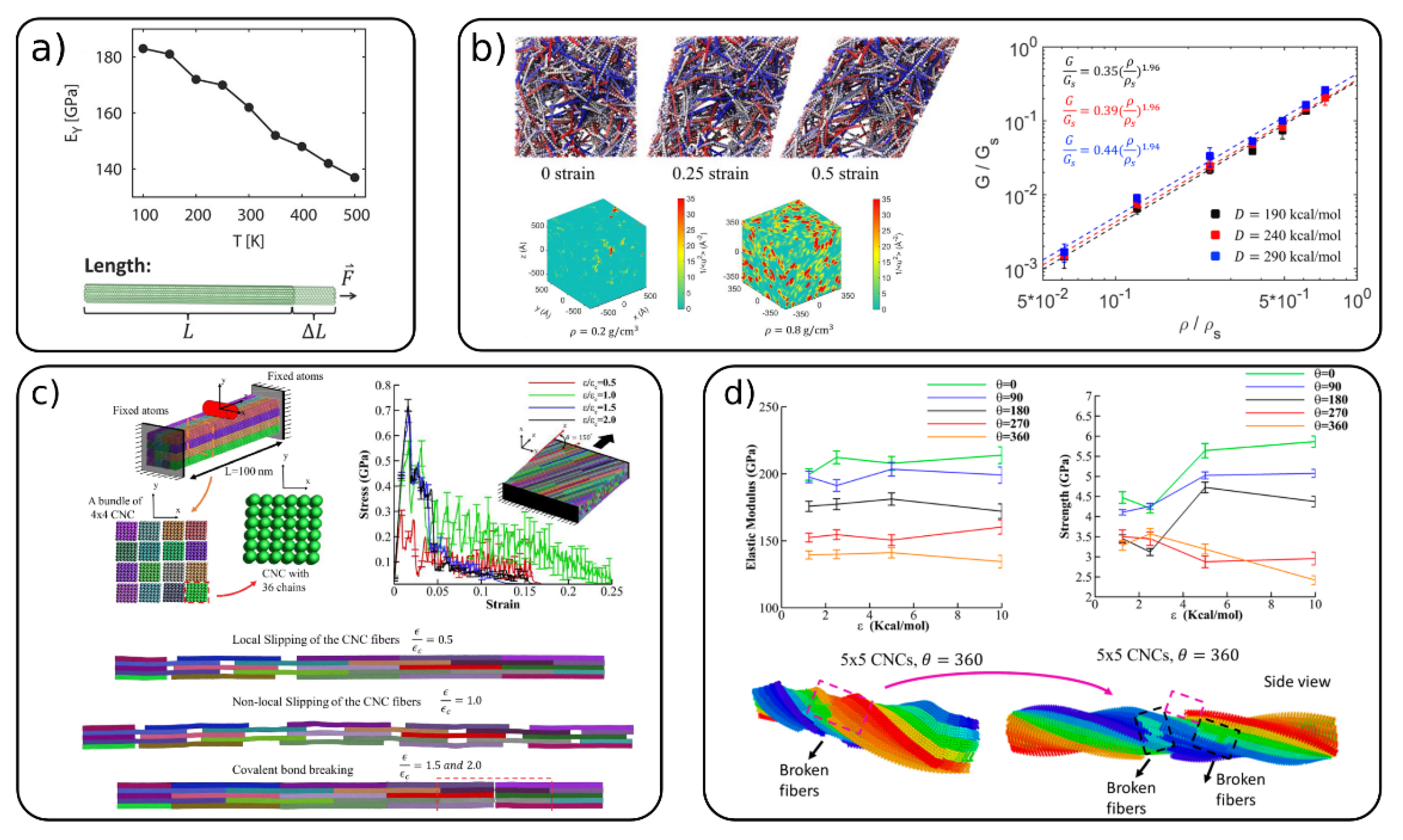
Figure 3. (a) The Young’s modulus of a single cellulose fiber for the realistic extension algorithm via covariance hessian (REACH) CG model and its variation with temperature, (adapted with permission from reference [40], 2012 American Chemical Society (ACS)) (b) shearing behavior of a CNC network: top—simulations snapshots at different strain; bottom—local molecular stiffness distribution for two different CNC density; right—relation between normalized shear modulus and CNC density, (adapted with permission from reference [60], 2020 Elsevier) (c) nano-indentation of CNC bundle, simulation snapshots and mechanical response of staggered and Bouligand CNC structures, (Adapted with permission from reference [53], 2019 Elsevier), (d) Elastic modulus and strength of CNC bundle (top) and simulation snapshots of the failure of 5 × 5 CNC bundle (bottom). (Adapted with permission from reference [52], 2019, MDPI).
Cellulose fibers and nanocrystals can assemble into a variety of structures such as bundles, brick-and-mortar structures, random cellulose networks and Bouligand structures (nematic phases). Qin et al. [61] studied the mechanical properties (elastic modulus, toughness and strength) of staggered CNC structures (nanopaper). They showed that the overlap length of CNCs is an important parameter affecting these properties. The critical length to maximize the mechanical properties is found to be in the range of tens to around a couple of hundreds of nanometers. Li and Xia [60] used the same CG model to investigate the mechanical properties of nanocellulose networks (see Figure 3b). The shear modulus (G) is shown to be strongly dependent on the mass density of CNCs in the network, while the cohesive energy between fibers has only little effect on G. The authors also calculated the local stiffness in these CNC networks, which was shown to be heterogeneously distributed across the network. This is evident from the “stiffness maps” (Figure 3b, boxes at the bottom) where red regions indicate areas with high stiffness (low mobility). The elastic modulus of cellulose networks with low CNC content (4.5% vol) were investigated by Mehandzhiyski et al. with the supra CG model. [54] The authors found values between 7.2 and 12.7 MPa closely reproducing typical values found in cellulose hydrogels.
Mechanical properties of various CNC structures (bundles, brick-and-mortar and Bouligand structures—Figure 3c) were studied by Shishehbor and Zavattieri [53] by the CG model they developed based on mechanical and interfacial properties. It was shown that the CNC bundle elasticity is increased, and its toughness is decreased with the increase in the cohesive (interfacial) interactions between the CNCs. The brick-and-mortar structures exhibit different failure mechanisms—localized slipping, nonlocal slipping and brittle failure, depending on the strength of the interfacial interactions. The Bouligand structures showed similar trends as the brick-and-mortar systems for the strength, toughness and elasticity. However, due to the different orientations of the staggered layers, the decrease in toughness due covalent bond breaking is reduced. The authors concluded that the twisted CNC/CNC interfaces show overall better mechanical properties than the untwisted interfaces. The same model was also used to investigate the effects of the bundle size and the twist of the whole bundle on the elastic modulus, strength, toughness, and failure strain for bundles of CNC (Figure 3d). [52] It was found that the increase in the bundle size and the twist angle decreases the mechanical properties due to bond breaking.
4.2. Conversion between Different Cellulose Allomorphs
The conversion of cellulose from crystalline to amorphous forms was studied by CG MD simulations in implicit [37] and explicit [44] water. The conversion between the forms was simulated with the thermodynamic integration (TI) method by applying a coupling parameter (λ) to the two states, where λ = 1 is the crystalline and λ = 0 is the amorphous form (Figure 4a). The parameter λ is coupled to the bonded and non-bonded interaction potentials. By monitoring several structural properties (Figure 4a), the authors found a transition between crystalline and amorphous cellulose around λ = 0.386 where the persistence length matches the experimental one. A comparison between the implicit and explicit solvents reveals that the explicit water stabilizes cellulose in the crystalline form and the cellulose–water interactions play a dominant role in the transition to the amorphous form.
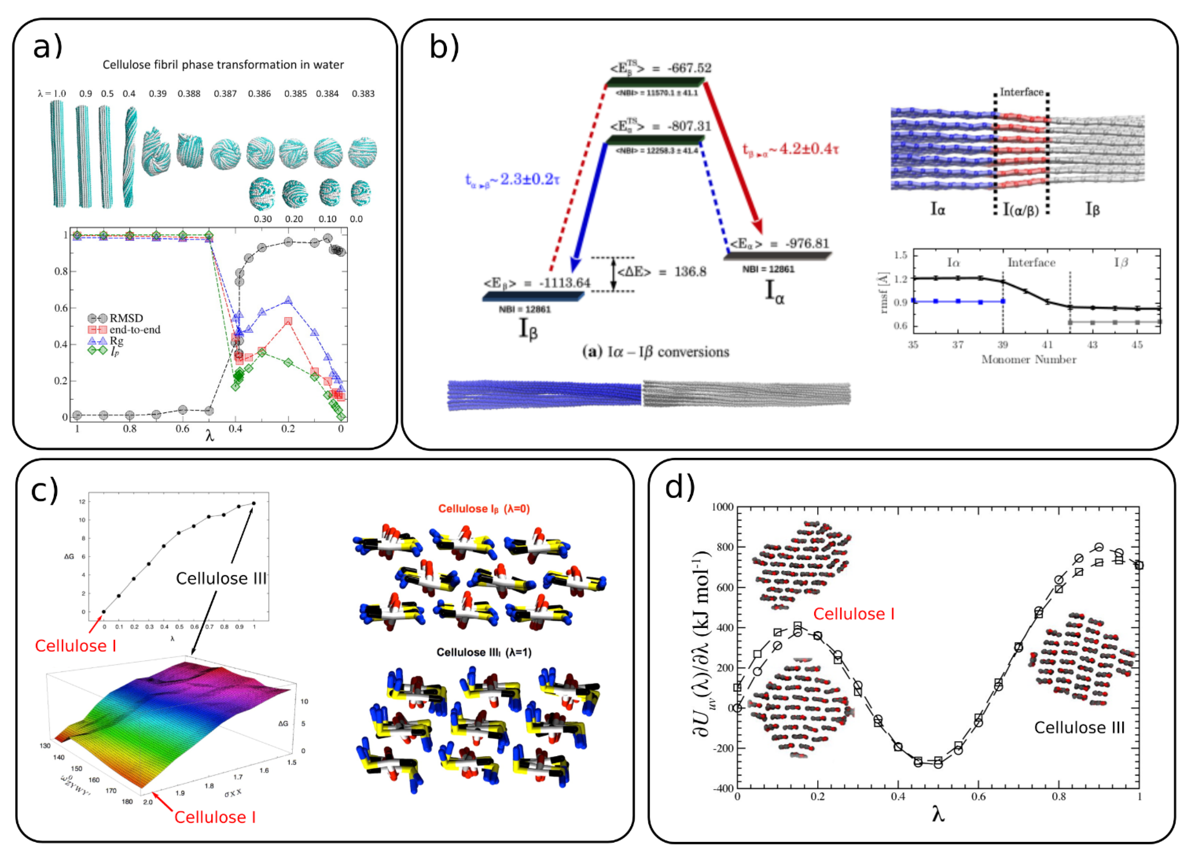
Figure 4. Conversion of cellulose between (a) crystalline and amorphous forms where the top panel shows the cellulose structure with varying λ (λ = 1 crystalline and λ = 0 amorphous) and bottom panel presents the root mean square displacement (RMSD), end-to-end distance, persistence length and radius of gyration for varying λ. (Adapted with permission from reference [44], 2014, American Chemical Society (ACS)), (b) cellulose Iβ→Iα transformation energy profile and co-existing Iα/Iβ crystalline form in one fibril (adapted with permission from reference [50], 2016, Springer), (c) energy profiles for cellulose conversion between I→IIII, where the respective structures are shown in the right panel (adapted with permission from reference [41], 2012, American Chemical Society (ACS)]), (d) energy profiles for cellulose I→IIII with their respective structures obtain from the simulations shown as insets (adapted with permission from reference [29], 2014, American Chemical Society (ACS)).
The conversion between different allomorphs, such as cellulose Iβ→Iα [50] and Iβ→IIII [29][41], was also studied with CG MD. Poma et al. have simulated the coexistence of the two forms (Iβ and Iα) in the same fibril, which shows a smooth transition region of around three glucose units (Figure 4b). They also showed, by using the TI simulations, that Iβ is the more stable allomorph than Iα. The energy difference between the two allomorphs was found to be 136.8 kcal/mol. The transformation of cellulose Iβ to cellulose IIII, depicted in Figure 4c,d, shows that the Iβ allomorph is more stable than IIII.
4.3. Cellulose-Cellulose Interactions and Self-Assembly of Cellulose Network
Cellulose nanocrystals and fibrils can self-assemble into different structures depending on their surface modifications. The surface modifications and ionic strength can induce attractive or repulsive interactions between CNCs [49][65]. Negatively charged CNC (TEMPO oxidized or sulfonated) in dispersion exhibit highly repulsive interactions, as illustrated in Figure 5a. However, with the increase in the ionic strength, these interactions can become even attractive, which induces the aggregation of CNC [49][66].
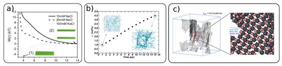
Figure 5. (a) Cellulose–cellulose potential of mean forces between two CNCs for different ionic strengths (adapted with permission from reference [49], 2016, Springer), (b) evolution of the CNC volume fraction (φ) as a function of the simulation time during water evaporation. The inset simulation snapshots show the initial and final structure with φ = 1 and φ = 4.5 vol%, respectively (adapted with permission from reference [54], 2020, Springer), (c) simulation snapshots of self-assembled structure of cellulose with chain length 20 and hydrogen bond strength εAD = 6.5 kcal/mol (adapted with permission from reference [56], 2020, American Chemical Society (ACS)).
A lower amount or absence of substitution for the surface hydroxyl groups also leads to an attractive interaction, and therefore to the self-assembly of cellulose particles [54][56][65]. An evolution of cellulose network formation with time and the CNC content of a native (no surface modifications) cellulose Iβ is shown in Figure 5b. From a dispersed state with around 1 wt% CNC, the system starts to form a highly percolated network even at low CNC content (~4.5 wt%) within 15 μs of simulation time. Such a percolated network of CNCs can be considered as a gel.
It is generally accepted that the attractive interactions between cellulose nanocrystals and fibrils is due to the formation of hydrogen bonds. The self-assembly of α-1,3glucans and CNC due to hydrogen bonding was recently modeled by CG simulations [56][62]. The strength of the hydrogen bonds and the effect of surface modifications on the assembly of CNC was investigated, revealing that highly ordered structures formed when the hydrogen bond strength was high (see Figure 5c). The effect of substitution to methylcellulose (MC) showed that substitution in the primary hydroxyl group (−O6H) lowers the amount of aggregates, thus increasing the water solubility of MC CNC.
4.4. Chiral Nematic Phases
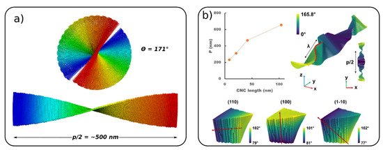
The right-handed twist of a single CNC giving rise to a left-handed twist of aggregated CNC is referred to as Bouligand structures or a chiral nematic phase [67]. The self-assembly of CNCs and formation of Boulgand structures is a particular challenge, which has not been fully explored yet by molecular simulations. However, two recent CG models of CNC were used to simulate chiral nematic ordering [54][55]. Mehandzhiyski et al. using the sCG model studied a chiral nematic ordering of a pre-assembled CNC structure showing a half pitch (rotation of 180° along the cholesteric phase) p/2 = 500 nm for native cellulose (Figure 6a). Rolland et al. [55] started from a completely flat arrangement of the cellulose nanocrystals and the right-hand twist of the 1D cholesteric ribbon naturally developed in the course of the simulations (Figure 6b). Figure 6b also presents the evolution of the pitch as a function of the CNC length for a cholesteric ribbon made of CNC with lengths of 100 nm. The pitch of the cholesteric phase shows an increase with the increase in the CNC length. The authors also simulated a CNC tactoid (ellipsoidal nanodroplet), which is believed to form during the initial stages of phase separation and formation of the nematic phase. These simulations present a first step towards an understanding of the formation of Bouligand structures of CNC. It should be noted here that Shishehbor and Zavattieri [53] studied the mechanical properties of Bouligand structures. However, these structures were pre-assembled and the focus in this study has been on the mechanical properties rather than on their formation.
4.5. Cellulose Composite Materials and Interactions with Other Molecules
In this section, we focus on cellulose usage in composite materials and on the interactions of cellulose with other molecules. In composite materials, cellulose was used as an additive, enhancing the mechanical properties or acting as a structural scaffold [58][68][69][70]. Martini CG modeling was used to simulate the morphology of a composite of cellulose with conductive polymer poly(3,4-ethylenedioxythiophene):poly(styrenesulfonate) (PEDOT:PSS). The modelling combined the otherwise independently developed models of the constituent polymers and cellulose [28][68][71][72]. The authors simulated the relevant experimental morphologies of PEDOT:PSS/CNC, highlighting the effects of different experimental conditions on the resulting morphology, leading to an inhomogeneous (granular) or homogeneous distribution of the polymers on the cellulose surface (Figure 7a). It was also shown that PEDOT is adsorbed mainly in a face-on configuration on the CNC surface. Another composite material studied by CG simulations is a blend of cellulose and polymer poly(methyl methacrylate) (PMMA) [58]. It was shown that, when added to PMMA, cellulose even in low quantities can improve the mechanical properties of the neat polymer. This was attributed to CNC percolation and PMMA “bridging” the individual CNC particles. The favorable interactions between PMMA and the carboxylic groups at the CNC interface were found to be an additional mechanism for the energy dissipation and increase in the toughness of the materials.
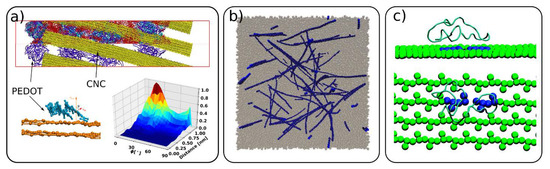
Figure 7. (a) Morphology of composite material of poly(3,4-ethylenedioxythiophene) and poly(styrenesulfonate) (PEDOT:PSS) and cellulose (yellow) and PEDOT adsorption on CNC surface (adapted with permission from reference [68], 2019, American Chemical Society (ACS)), (b) composite of cellulose (blue) and poly(methyl methacrylate) (gray) (adapted with permission from reference [58], 2015, American Chemical Society (ACS)), (c) carbohydrate binding module (CBM) of Cel7A interaction with cellulose surface where in blue is highlighted the hydrolized glucosidic bond (adapted with permission from reference [36], 2009, American Chemical Society (ACS)).
Cellulose interactions with other macromolecules, such as proteins [47] and enzymes [28][36], have also been investigated by CG simulations. Enzymes, such as Trichoderma reesei cellobiohydrolase (CBH) I (Cel7A), are responsible for cellulose hydrolysis, and thus are industrially important for cellulose decomposition. The translational motion and thermodynamic driving forces of the carbohydrate binding module (CBM) of Cel7A on the cellulose surface was investigated with the Martini CG model [28] and mixed atomistic–CG simulations [36], respectively (Figure 7c). Specific CG models for cellulose interacting with xylan [46] and ionic liquids [57] were also developed and provided a fundamental insight into the interactions between the different species.
This entry is adapted from the peer-reviewed paper 10.3390/polysaccharides2020018
References
- Klemm, D.; Heublein, B.; Fink, H.-P.; Bohn, A. Cellulose: Fascinating Biopolymer and Sustainable Raw Material. Angew. Chem. Int. Ed. 2005, 44, 3358–3393.
- Eyley, S.; Thielemans, W. Surface Modification of Cellulose Nanocrystals. Nanoscale 2014, 6, 7764.
- Dufresne, A. Nanocellulose: A New Ageless Bionanomaterial. Mater. Today 2013, 30, 1704285.
- Jarvis, M.C. Structure of Native Cellulose Microfibrils, the Starting Point for Nanocellulose Manufacture. Philos. Trans. R. Soc. A Math. Phys. Eng. Sci. 2018, 376, 20170045.
- Ding, S.-Y.; Zhao, S.; Zeng, Y. Size, Shape, and Arrangement of Native Cellulose Fibrils in Maize Cell Walls. Cellulose 2014, 2, 1863–1871.
- Nixon, B.T.; Mansouri, K.; Singh, A.; Du, J.; Davis, J.K.; Lee, J.-G.; Slabaugh, E.; Vandavasi, V.G.; O’Neill, H.; Roberts, E.M.; et al. Comparative Structural and Computational Analysis Supports Eighteen Cellulose Synthases in the Plant Cellulose Synthesis Complex. Sci. Rep. 2016, 6, 28696.
- Ling, S.; Kaplan, D.L.; Buehler, M.J. Nanofibrils in Nature and Materials Engineering. Nat. Rev. Mater. 2018, 3, 1–15.
- Trache, D.; Hussin, M.H.; Haafiz, M.K.M.; Thakur, V.K. Recent Progress in Cellulose Nanocrystals: Sources and Production. Nanoscale 2017, 9, 1763–1786.
- Moon, R.J.; Martini, A.; Nairn, J.; Simonsenf, J.; Youngblood, J. Cellulose Nanomaterials Review: Structure, Properties and Nanocomposites. Chem. Soc. Rev. 2011, 40, 3941–3994.
- Shankaran, D.R. Chapter 14—Cellulose Nanocrystals for Health Care Applications. In Applications of Nanomaterials; Mohan Bhagyaraj, S., Oluwafemi, O.S., Kalarikkal, N., Thomas, S., Eds.; Micro and Nano Technologies; Woodhead Publishing: Cambridge, UK, 2018; pp. 415–459. ISBN 978-0-08-101971-9.
- Fan, J.; Zhang, S.; Li, F.; Shi, J. Cellulose-Based Sensors for Metal Ions Detection. Cellulose 2020, 27, 5477–5507.
- Fan, J.; Zhang, S.; Li, F.; Yang, Y.; Du, M. Recent Advances in Cellulose-Based Membranes for Their Sensing Applications. Cellulose 2020, 27, 9157–9179.
- Chen, W.; Yu, H.; Lee, S.-Y.; Wei, T.; Li, J.; Fan, Z. Nanocellulose: A Promising Nanomaterial for Advanced Electrochemical Energy Storage. Chem. Soc. Rev. 2018, 47, 2837.
- Zhang, L.; Han, J.; Wang, H.; Car, R.; Weinan, E. DeePCG: Constructing Coarse-Grained Models via Deep Neural Networks. J. Chem. Phys. 2018, 149, 034101.
- Chakraborty, M.; Xu, C.; White, A.D. Encoding and Selecting Coarse-Grain Mapping Operators with Hierarchical Graphs. J. Chem. Phys. 2018, 149, 134106.
- Li, Z.; Wellawatte, G.P.; Chakraborty, M.; Gandhi, H.A.; Xu, C.; White, A.D. Graph Neural Network Based Coarse-Grained Mapping Prediction. Chem. Sci. 2020, 11, 9524–9531.
- Lyubartsev, A.P.; Laaksonen, A. Calculation of Effective Interaction Potentials from Radial Distribution Functions: A Reverse Monte Carlo Approach. Phys. Rev. E 1995, 52, 3730–3737.
- Lyubartsev, A.P.; Naômé, A.; Vercauteren, D.P.; Laaksonen, A. Systematic Hierarchical Coarse-Graining with the Inverse Monte Carlo Method. J. Chem. Phys. 2015, 143, 243120.
- Shell, M.S. The Relative Entropy Is Fundamental to Multiscale and Inverse Thermodynamic Problems. J. Chem. Phys. 2008, 129, 144108.
- Izvekov, S.; Voth, G.A. A Multiscale Coarse-Graining Method for Biomolecular Systems. J. Phys. Chem. B 2005, 109, 2469–2473.
- Izvekov, S.; Voth, G.A. Multiscale Coarse Graining of Liquid-State Systems. J. Chem. Phys. 2005, 123, 134105.
- Moritsugu, K.; Smith, J.C. Coarse-Grained Biomolecular Simulation with REACH: Realistic Extension Algorithm via Covariance Hessian. Biophys. J. 2007, 93, 3460–3469.
- Noid, W.G. Perspective: Coarse-Grained Models for Biomolecular Systems. J. Chem. Phys. 2013, 139, 090901.
- Brini, E.; Algaer, E.A.; Ganguly, P.; Li, C.; Rodríguez-Ropero, F.; van der Vegt, N.F.A. Systematic Coarse-Graining Methods for Soft Matter Simulations—A Review. Soft Matter 2013, 9, 2108–2119.
- Peter, C.; Kremer, K. Multiscale Simulation of Soft Matter Systems—from the Atomistic to the Coarse-Grained Level and Back. Soft Matter 2009, 5, 4357.
- Marrink, S.J.; Risselada, H.J.; Yefimov, S.; Tieleman, D.P.; de Vries, A.H. The MARTINI Force Field: Coarse Grained Model for Biomolecular Simulations. J. Phys. Chem. B. 2007, 111, 7812–7824.
- López, C.A.; Rzepiela, A.J.; de Vries, A.H.; Dijkhuizen, L.; Hünenberger, P.H.; Marrink, S.J. Martini Coarse-Grained Force Field: Extension to Carbohydrates. J. Chem. Theory Comput. 2009, 5, 3195–3210.
- Wohlert, J.; Berglund, L.A. A Coarse-Grained Model for Molecular Dynamics Simulations of Native Cellulose. J. Chem. Theory Comput. 2011, 7, 753–760.
- López, C.A.; Bellesia, G.; Redondo, A.; Langan, P.; Chundawat, S.P.S.; Dale, B.E.; Marrink, S.J.; Gnanakaran, S. MARTINI Coarse-Grained Model for Crystalline Cellulose Microfibers. J. Phys. Chem. B 2015, 119, 465–473.
- Shivgan, A.T.; Marzinek, J.K.; Huber, R.G.; Krah, A.; Henchman, R.H.; Matsudaira, P.; Verma, C.S.; Bond, P.J. Extending the Martini Coarse-Grained Force Field to N -Glycans. J. Chem. Inf. Model. 2020, 60, 3864–3883.
- Molinero, V.; Goddard, W.A. M3B: A Coarse Grain Force Field for Molecular Simulations of Malto-Oligosaccharides and Their Water Mixtures. J. Phys. Chem. B 2004, 108, 1414–1427.
- Molinero, V.; Çaǧın, T.; Goddard, W.A. Mechanisms of Nonexponential Relaxation in Supercooled Glucose Solutions: The Role of Water Facilitation. J. Phys. Chem. A 2004, 108, 3699–3712.
- Queyroy, S.; Neyertz, S.; Brown, D.; Müller-Plathe, F. Preparing Relaxed Systems of Amorphous Polymers by Multiscale Simulation: Application to Cellulose. Macromolecules 2004, 37, 7338–7350.
- Molinero, V.; Goddard, W.A. Microscopic Mechanism of Water Diffusion in Glucose Glasses. Phys. Rev. Lett. 2005, 95, 045701.
- Liu, P.; Izvekov, S.; Voth, G.A. Multiscale Coarse-Graining of Monosaccharides. J. Phys. Chem. B 2007, 111, 11566–11575.
- Bu, L.; Beckham, G.T.; Crowley, M.F.; Chang, C.H.; Matthews, J.F.; Bomble, Y.J.; Adney, W.S.; Himmel, M.E.; Nimlos, M.R. The Energy Landscape for the Interaction of the Family 1 Carbohydrate-Binding Module and the Cellulose Surface Is Altered by Hydrolyzed Glycosidic Bonds. J. Phys. Chem. B 2009, 113, 10994–11002.
- Srinivas, G.; Cheng, X.; Smith, J.C. A Solvent-Free Coarse Grain Model for Crystalline and Amorphous Cellulose Fibrils. J. Chem. Theory Comput. 2011, 7, 2539–2548.
- Hynninen, A.-P.; Matthews, J.F.; Beckham, G.T.; Crowley, M.F.; Nimlos, M.R. Coarse-Grain Model for Glucose, Cellobiose, and Cellotetraose in Water. J. Chem. Theory Comput. 2011, 7, 2137–2150.
- Markutsya, S.; Kholod, Y.A.; Devarajan, A.; Windus, T.L.; Gordon, M.S.; Lamm, M.H. A Coarse-Grained Model for β-d-Glucose Based on Force Matching. Chem. Acc. 2012, 131, 1162.
- Glass, D.C.; Moritsugu, K.; Cheng, X.; Smith, J.C. REACH Coarse-Grained Simulation of a Cellulose Fiber. Biomacromolecules 2012, 13, 2634–2644.
- Bellesia, G.; Chundawat, S.P.S.; Langan, P.; Redondo, A.; Dale, B.E.; Gnanakaran, S. Coarse-Grained Model for the Interconversion between Native and Liquid Ammonia-Treated Crystalline Cellulose. J. Phys. Chem. B 2012, 116, 8031–8037.
- Wu, S.; Zhan, H.; Wang, H.; Ju, Y. Secondary Structure Analysis of Native Cellulose by Molecular Dynamics Simulations with Coarse Grained Model. Chin. J. Chem. Phys. 2012, 25, 191–198.
- Markutsya, S.; Devarajan, A.; Baluyut, J.Y.; Windus, T.L.; Gordon, M.S.; Lamm, M.H. Evaluation of Coarse-Grained Mapping Schemes for Polysaccharide Chains in Cellulose. J. Chem. Phys. 2013, 138, 214108.
- Srinivas, G.; Cheng, X.; Smith, J.C. Coarse-Grain Model for Natural Cellulose Fibrils in Explicit Water. J. Phys. Chem. B 2014, 118, 3026–3034.
- Rusu, V.H.; Baron, R.; Lins, R.D. PITOMBA: Parameter Interface for Oligosaccharide Molecules Based on Atoms. J. Chem. Theory Comput. 2014, 10, 5068–5080.
- Li, L.; Pérré, P.; Frank, X.; Mazeau, K. A Coarse-Grain Force-Field for Xylan and Its Interaction with Cellulose. Carbohydr. Polym. 2015, 127, 438–450.
- Poma, A.B.; Chwastyk, M.; Cieplak, M. Polysaccharide-Protein Complexes in a Coarse-Grained Model. J. Phys. Chem. B 2015, 119, 12028–12041.
- Fan, B.; Maranas, J.K. Coarse-Grained Simulation of Cellulose Iβ with Application to Long Fibrils. Cellulose 2015, 22, 31–44.
- Phan-Xuan, T.; Thuresson, A.; Skepö, M.; Labrador, A.; Bordes, R.; Matic, A. Aggregation Behavior of Aqueous Cellulose Nanocrystals: The Effect of Inorganic Salts. Cellulose 2016, 23, 3653–3663.
- Poma, A.B.; Chwastyk, M.; Cieplak, M. Coarse-Grained Model of the Native Cellulose I-Alpha and the Transformation Pathways to the I-Beta Allomorph. Cellulose 2016, 23, 1573–1591.
- Poma, A.; Chwastyk, M.; Cieplak, M. Elastic Moduli of Biological Fibers in a Coarse-Grained Model: Crystalline Cellulose and Beta-Amyloids. Phys. Chem. Chem. Phys. 2017, 19, 28195–28206.
- Ramezani, M.G.; Golchinfar, B. Mechanical Properties of Cellulose Nanocrystal (CNC) Bundles: Coarse-Grained Molecular Dynamic Simulation. J. Compos. Sci. 2019, 3, 57.
- Shishehbor, M.; Zavattieri, P.D. Effects of Interface Properties on the Mechanical Properties of Bio-Inspired Cellulose Nanocrystal (CNC)-Based Materials. J. Mech. Phys. Solids 2019, 124, 871–896.
- Mehandzhiyski, A.Y.; Rolland, N.; Garg, M.; Wohlert, J.; Linares, M.; Zozoulenko, I. A Novel Supra Coarse-Grained Model for Cellulose. Cellulose 2020, 27, 4221–4234.
- Rolland, N.; Mehandzhiyski, A.Y.; Garg, M.; Linares, M.; Zozoulenko, I.V. New Patchy Particle Model with Anisotropic Patches for Molecular Dynamics Simulations: Application to a Coarse-Grained Model of Cellulose Nanocrystal. J. Chem. Theory Comput. 2020, 16, 3699–3711.
- Wu, Z.; Beltran-Villegas, D.J.; Jayaraman, A. Development of a New Coarse-Grained Model to Simulate Assembly of Cellulose Chains Due to Hydrogen Bonding. J. Chem. Theory Comput. 2020, 16, 4599–4614.
- Reyes, G.; Aguayo, M.G.; Fernández Pérez, A.; Pääkkönen, T.; Gacitúa, W.; Rojas, O.J. Dissolution and Hydrolysis of Bleached Kraft Pulp Using Ionic Liquids. Polymers 2019, 11, 673.
- Dong, H.; Sliozberg, Y.R.; Snyder, J.F.; Steele, J.; Chantawansri, T.L.; Orlicki, J.A.; Walck, S.D.; Reiner, R.S.; Rudie, A.W. Highly Transparent and Toughened Poly(Methyl Methacrylate) Nanocomposite Films Containing Networks of Cellulose Nanofibrils. Acs Appl. Mater. Interfaces 2015, 7, 25464–25472.
- Ray, U.; Pang, Z.; Li, T. Mechanics of Cellulose Nanopaper Using a Scalable Coarse-Grained Modeling Scheme. Cellulose 2021.
- Li, Z.; Xia, W. Coarse-Grained Modeling of Nanocellulose Network towards Understanding the Mechanical Performance. Extrem. Mech. Lett. 2020, 40, 100942.
- Qin, X.; Feng, S.; Meng, Z.; Keten, S. Optimizing the Mechanical Properties of Cellulose Nanopaper through Surface Energy and Critical Length Scale Considerations. Cellulose 2017, 24, 3289–3299.
- Beltran-Villegas, D.J.; Intriago, D.; Kim, K.H.C.; Behabtu, N.; Londono, J.D.; Jayaraman, A. Coarse-Grained Molecular Dynamics Simulations of α-1,3-Glucan. Soft Matter 2019, 15, 4669–4681.
- Kern, N.; Frenkel, D. Fluid–Fluid Coexistence in Colloidal Systems with Short-Ranged Strongly Directional Attraction. J. Chem. Phys. 2003, 118, 9882–9889.
- Shishehbor, M.; Dri, F.L.; Moon, R.J.; Zavattieri, P.D. A Continuum-Based Structural Modeling Approach for Cellulose Nanocrystals (CNCs). J. Mech. Phys. Solids 2018, 111, 308–332.
- Garg, M.; Linares, M.; Zozoulenko, I. Theoretical Rationalization of Self-Assembly of Cellulose Nanocrystals: Effect of Surface Modifications and Counterions. Biomacromolecules 2020, 21, 3069–3080.
- Benselfelt, T.; Nordenström, M.; Hamedi, M.M.; W\aagberg, L. Ion-Induced Assemblies of Highly Anisotropic Nanoparticles Are Governed by Ion-Ion Correlation and Specific Ion Effects. Nanoscale 2019, 11, 3514–3520.
- Parker, R.M.; Guidetti, G.; Williams, C.A.; Zhao, T.; Narkevicius, A.; Vignolini, S.; Frka-Petesic, B. The Self-Assembly of Cellulose Nanocrystals: Hierarchical Design of Visual Appearance. Adv. Mater. 2018, 30, 1704477.
- Mehandzhiyski, A.Y.; Zozoulenko, I. Computational Microscopy of PEDOT:PSS/Cellulose Composite Paper. ACS Appl. Energy Mater. 2019, 2, 3568–3577.
- Peterson, A.; Mehandzhiyski, A.Y.; Svenningsson, L.; Ziolkowska, A.; Kádár, R.; Lund, A.; Sandblad, L.; Evenäs, L.; Lo Re, G.; Zozoulenko, I.; et al. A Combined Theoretical and Experimental Study of the Polymer Matrix Mediated Stress Transfer in a Cellulose Nanocomposite. Macromolecules 2021.
- Belaineh, D.; Andreasen, J.W.; Palisaitis, J.; Malti, S.; Håkansson, K.; Wågberg, L.; Crispin, X.; Engquist, I.; Berggren, M. Controlling the Organization of PEDOT: PSS on Cellulose Structures. Acs Appl. Polym. Mater. 2019, 1, 2342–2351.
- Modarresi, M.; Franco-Gonzalez, J.F.; Zozoulenko, I. Morphology and Ion Diffusion in PEDOT:Tos. A Coarse Grained Molecular Dynamics Simulation. Phys. Chem. Chem. Phys. 2018, 20, 17188.
- Holm, M.V.C.; Smiatek, J. Coarse-Grained Simulations of Polyelectrolyte Complexes: MARTINI Models for Poly(Styrene Sulfonate) and Poly(Diallyldimethylammonium). J. Chem. Phys. 2015, 143, 243151.
This entry is offline, you can click here to edit this entry!