Human activities and climate change constitute the contemporary catalyst for natural processes and their impacts, i.e., geo-environmental hazards. Globally, natural catastrophic phenomena and hazards, such as drought, soil erosion, quantitative and qualitative degradation of groundwater, frost, flooding, sea level rise, etc., are intensified by anthropogenic factors. Thus, they present rapid increase in intensity, frequency of occurrence, spatial density, and significant spread of the areas of occurrence. The impact of these phenomena is devastating to human life and to global economies, private holdings, infrastructure, etc., while in a wider context it has a very negative effect on the social, environmental, and economic status of the affected region. Geospatial technologies including Geographic Information Systems, Remote Sensing—Earth Observation as well as related spatial data analysis tools, models, databases, contribute nowadays significantly in predicting, preventing, researching, addressing, rehabilitating, and managing these phenomena and their effects.
- environmental monitoring
- climate change
- geohazards
1. Drought Monitoring
With its stability and durability, nature can introduce extreme changes in the variables and factors of human systems. Extreme changes or extreme events, such as earthquakes, floods, and droughts, often called natural hazards, can present insurmountable obstacles and difficulties in how human societies deal with them [1][2][3][4][5]. In this context, it is argued that droughts are one of many natural hazards that can affect domestic use and irrigation—in other words, the water supply of an area [6][7]. The current trend among broad technical and professional circles, administrators, politicians, and decision-makers and generally among common citizens is to regard drought as something transient, a random and remote risk that requires only an extraordinary mobilization [8][9]. However, the accumulated experience of scientific research and observations in recent decades shows that droughts are inevitable, as these phenomena appear to be inescapable and permanent elements of the global climate [8][10][11][12][13][14]. Drought issues can turn into a water crisis and will play a crucial role in the next years in defining both development and environmental policies on a world level [15][16][17]. As far as Europe is concerned, the droughts in Greece in 1989–1993, in Spain in 2003, in France in 2005, and again in Greece in 2007–2008, confirm this trend, as well as the urgent need to implement common strategies to the problem across Europe and not just in the Mediterranean countries [1][11][18][19][20][21][22][23][24]. The next figure (Figure 1) presents such a context [21].
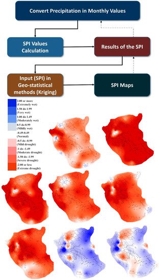
Figure 1. Example of Geographic Information Systems (GIS) technique for monitoring/simulate drought [21].
Drought and its consequences must be recognized and taken into account from the early stages of water resources planning and management efforts [25][26][27][28][29]. Accordingly, measures and efforts to tackle droughts should begin by studying the phenomenon’s dimensions [1][30][31][32]. Functional definitions allow the determination of the beginning and end, as well as the degree of severity of drought [1][11][33][34]. These definitions are categorized based on four different approaches: meteorological, hydrological, agricultural, and socioeconomic drought. GIS and Expert Systems (E.S.) can respond timely to identify and recognize drought events over large areas through satellite data, gridded datasets, and measured values from meteorological stations. However, the calculation of Drought Risk and Vulnerability Assessment require spatial data on specific time step (monthly or yearly). Thus, using geoinformation solutions improve the observation visualization of drought hazards. [5][10][11][12][14][20][35][36][37].
Drought is a temporary state (months/years), instead of aridity, which is a permanent climate feature [38][39]. Additionally, seasonal drought, i.e., a well-defined dry season, must be distinguished from the drought that occurs with different characteristics [5][6]. There is considerable confusion between scientists and policymakers about diversifying these terms. A typical example is the Greek territory, especially in the island regions, where the rainfall season begins in October and ends in April [19][21][22]. Thus, a large part of the islands appears barren, and drought is an inevitable climate feature. However, the seasonal drought on these islands is almost certain to occur over time due to the failure to meet water needs over a given time horizon. Drought usually occurs when rainfall in a region is less than average and is followed by large evaporation rates for prolonged periods [20][37][40][41][42]. The drought varies from other natural disasters because of its leisureliness and long duration. In most cases, drought is caused either by a decrease in rainfall or a shortage of water resources reserves. The concept of deficiency is relevant and determined by a specific water demand by sector or by specific activities. Nevertheless, drought analyses and drought assessments should include all the available data from the investigated study area. These results composing drought indices (indicators or indexes) were visualized on a GIS environment to portray spatial distribution. There are efforts and they use geo-statistical techniques to transform the point values form meteorological stations to a spatial distribution in a specific time frame, namely, kriging and co-kriging methods and Inverse Distance Weighting (IDW) are the most common approaches it is referred to as having a better fit for indices or climate parameters [1][4][7][10][14][43].
To address drought phenomena, the development of a strategy and a Master Plan of these phenomena is recommended as an effective means of improving the ability to assess and respond to state mechanisms for action. Unanimity between state agencies and private and public interest groups is also an important part of the process. Composite indicators and indices can help recognize a drought promptly and achieve this goal. Additionally, in combination with forecasting models, a short-term prediction of the phenomenon and its effects can be successfully made for decision-makers to be able to better prepare by reducing or minimizing the effects and reaction time to them. An important helper in this direction is the promotion and integration of contingency planning.
2. Soil Erosion Monitoring
Soil erosion is a complex and dynamic phenomenon that affects many areas around the world. It is one of the most serious problems of land degradation and a major source of environmental deterioration, as it is the largest environmental problem the world is facing after population growth. Indicatively, it is reported that the United States loses soil 10 times faster than the rate of natural replenishment, while the corresponding loss for China and India is 30–40 times faster [44].
Worldwide, the total area of land affected by water erosion is 10,940,000 km2, of which 7,510,000 km2 are significantly degraded [45]. The annual sediment transport to the ocean from rivers around the world has been estimated to be 15 to 30 billion tonnes [46][47]. In addition, soil erosion affects the geomorphological characteristics of an area in terms of soil fertility, agricultural productivity, water quality, water reservoir capacity, and the evolution of coastal areas in sedimentary environments [48][49][50].
The current evolution of the erosion phenomenon is directly related to global warming, which results in a more intense hydrological cycle in several regions, including more total rainfalls and more frequent events of high intensity rainfall (combined or not). These changes in rainfall, as well as changes in temperature, solar radiation, and atmospheric CO2 concentrations, have significant effects on soil erosion rates. In general, the processes associated with the effects of climate change on soil erosion by water are complex and include changes in the volume and intensity of rainfall, number of days of rainfall, ratio between rain and snow, production of biomass from plants, decomposition rates of vegetable residues, evapotranspiration rates, and land use changes that are necessary to adapt to a new climate regime [51].
In addition, degradation of agricultural land by soil erosion is also a global phenomenon leading to the loss of nutrient-rich surface soil, increased runoff in the more impermeable layer of the ground and reduced availability of water to plants [52]. About 85% of soil degradation worldwide is associated with soil erosion and causes up to 17% reduction in crop productivity [53].
Effective monitoring, modeling, and analysis of the soil erosion phenomenon can provide information on the current erosion state, trends, and allow the analysis of different scenarios [52]. Furthermore, these actions can be important sources of information for land management decisions through the development of alternative land use scenarios and the evaluation of their results [54]. Quantitative monitoring and evaluation [55] is often required to extract the extent and magnitude of soil erosion problems in order to develop sound regional management strategies along with field measurements.
Soil erosion monitoring and analysis models are classified [56] into three main categories: empirical, conceptual (partly empirical/mixed) and physical. Examples of the three categories include the empirical model USLE and its modifications, the conceptual ANSWERS (Areal Nonpoint Source Watershed Environment Response Simulation), CREAMS (Chemicals, Runoff and Erosion from Agricultural Management Systems), and MODANSW (Modified ANSWERS), as well as the physical models EUROSEM (European Soil Erosion Model) and MIKE SHE (“Systeme Hydrologique Europeen” or European Hydrological System). Since 1930s, soil experts and decision-makers have been developing and using erosion models to monitor and calculate soil loss [57]. Over 80 erosion models have been created over the last fifty years [58].
One of the most widely used empirical models for monitoring and estimating erosion is the Universal Soil Loss Equation (USLE) model developed by Wischmeier and Smith in 1965, based on soil erosion measurements in the USA [57]. It has been developed mainly for the assessment of soil erosion on arable land or on slightly sloping topographies and is still used in a large number of studies to estimate soil loss [52]. With the revised version RUSLE, which takes into account the upstream areas that contribute to the downstream surface runoff and is thus considered to have better predictability than USLE [59], and modified version MUSLE [57][60][61], USLE is still widely used in soil loss assessment studies and is the most common tool for large-scale soil erosion assessment and monitoring in Europe [62][63][64][65].
In recent years, with the development and significant evolutions in GIS and remote sensing, as well as the progress made in computing power, efforts to spatially model soil erosion have been intensified and greatly upgraded [66]. The widespread dissemination of GIS and the use of satellite data has greatly facilitated the development of erosion models, since they allow the use of multiple data sources, easy modification of the structure of erosion models and unconditional reshaping of their scale [67][68]. The use of conventional methods for monitoring and assessing the risk of soil erosion is costly and time consuming. The integration of existing soil erosion models, field data and data provided by remote sensing technologies through the use of GIS has proved to be particularly advantageous, while enabling the spatial distribution of erosion to be presented through hazard maps, which are necessary for the design of protective measures [50][52][65][69][70][71].
The importance of continuous monitoring of soil erosion and application of integrated river basin management practices has been enhanced by the independent use of remote sensing data, such as aerial photos, LiDAR, UAV, and satellite data such as Landsat (ETM +, TM, MSS), IRS-P6 LISS (III, IV), ASTER GDEM, GeoEye, QuickBird, WorldView, MODIS, Hyperion, etc., but also by their combined analysis and evaluation with other types of data, such as rain gauges, soil samples, topographic maps, etc., in GIS environment [72][73][74][75][76][77][78][79][80][81][82]. A typical example of the above is the soil erosion risk mapping on a monthly basis by Nigel et al. [83] for the Mauritius region via GIS, decision rules, rainfall, and soil data, and SPOT satellite imagery. They developed the MauSERM model, which produces high resolution soil erosion monitoring maps for the whole area of Mauritius every month.
The combined use of remote sensing data (and indicators derived by these like NDVI), GIS and soil loss assessment models, such as USLE, RUSLE, RUSLE3D (a modification of RUSLE for composite soil), USPED (Unit Stream Power-based Erosion Deposition), PESERA (Pan-European Soil Erosion Risk Assessment), etc., has proven to be extremely important and effective in monitoring and predicting soil erosion [52][84][85][86][87][88][89][90][91][92][93][94][95][96][97][98][99][100]. A good and recent example supporting the previous argument is the implementation by Karydas et al. [101] of the G2 soil erosion model in five study areas in south-eastern Europe and Cyprus aiming to estimate soil loss on a monthly basis. This model operates in a GIS environment utilizing a wealth of satellite data such as Sentinel-2, MERIS, PROBA-V and SPOT-VGT. Based also on the above, a very useful reference would be the work of Leh et al. [102], who created scenarios for predicting future land use allocation and soil erosion levels for a US catchment area for 2030. This research combined remote sensing, GIS and modeling techniques and created land use maps through analysis of Landsat satellite images every five years for a period of 20 years (1986–2006). The studies were based on these maps for the synthesis of future scenarios that predict an increase in urbanization with a consequent increase in erosion risk for the study area.
Steps forward in the development of the previous logic were the utilization of the aforementioned data, models and methods along with the use of other techniques such as Frequency Ratio (FR), Analytical Hierarchy Process (AHP), Logistic Regression (LR), Multiple Linear Regression (MLR), Potential Erosion Index (PEI), Sediment Delivery Ratio (SDR), the GIS model GWLF (Generalized Watershed Loading Function), the TLSD (Transport Limited Sediment Delivery) function, etc. [103][104][105][106][107]. A worth noting and recent example is the work of Macedo et al. [108], who developed the Environmental Fragility Index (EFI) through GIS procedures and its ability to monitor and predict sediment deposition was evaluated on 148 rivers in Brazil. The index takes into account geoclimatic factors as well as anthropogenic pressures and utilizes geospatial, rainfall and Landsat TM satellite data.
In conclusion, taking into consideration all previous references, GIS and Remote Sensing are proven very useful tools with great potential in monitoring and estimating soil erosion reliably. These can be based on either models as for example USLE/RUSLE [91][109][110][111][112][113], or in other methods like for example Multi-Criteria Evaluation Techniques—MCE [114][115][116][117][118][119][120][121], or in combinations of the above.
Finally, spatial information analysis is an ever-evolving approach capable of monitoring evaluating, managing and analyzing the complex problems, such as soil erosion, of river basins and lake basins. In recent years, GIS has proven to be a good alternative as they are better decision support tools in soil monitoring, planning, management and sustainable development.
3. Groundwater Monitoring
Groundwater is one of the most valuable natural resources and is related, directly, to human health, economic development, and ecological diversity [122]. They are a vital resource for reliable and affordable drinking water supply in urban and rural environments and play a fundamental role in human well-being, sustainable agriculture, and the conservation of aquatic and terrestrial ecosystems [123]. Groundwater quality is usually very good, as it is filtered naturally through the soil and is clear, colorless, and free of microbial contamination, requiring minimal treatment [124].
Effective groundwater management and monitoring is of particular importance in areas with hard rocky soil, which are deprived almost everywhere and permanently of surface water. In these areas, where ever-growing human populations live, finding water supply zones is increasingly difficult [125]. In addition, in many areas groundwater availability is limited, and aquifer development is mainly associated with fractured and disintegrated horizons and secondary porosity created [126]. Moreover, exposure to various pollutants can render groundwater unsuitable for consumption and can endanger human life, fauna, and the environment [127].
Assessing the impact of climate change on a country’s water resources is the most important assessment that has to be carried out before planning any long-term water potential project. Numerous studies have been conducted worldwide on the trends of river flows in relation to water filtration in the face of climate change and potential pressures on groundwater aquifers [128]. In recent years, researchers around the world, have conducted numerous studies to assess groundwater reserves and groundwater aquifers, as sustainable groundwater management is increasingly necessary. Investigation of groundwater presence and delineation of groundwater aquifers can be achieved by indirectly analyzing some directly observed soil characteristics, such as tectonics [129].
Unlike traditional methods, remote sensing (RS) technology, with the benefits of spatial, spectral, and temporal data availability covering large and inaccessible areas in a short period of time, has proved to be a very useful tool for evaluation, monitoring and the management of groundwater resources [130][131]. In addition, it is widely used to map land surface features (such as linear tectonic elements, lithology, etc.), as well as to monitor groundwater supply zones [129].
Hydrogeological interpretation of satellite data has proven to be a valuable research tool in areas where little geological and cartographic information is available (or not accurate) as well as inaccessible areas [130]. Since satellite sensors cannot directly detect groundwater, the presence of groundwater results from the interpretation of different surface features derived from satellite images, such as geology, soil geomorphology, soil characteristics (texture, roughness, etc.), land uses/land cover, surface water bodies, etc. [132][133]. In recent years, the widespread use of satellite data in combination with conventional maps and corrected terrain data has facilitated the extraction of baseline information [134][135][136][137][138][139].
Alongside remote sensing, GSPs have emerged as powerful tools for spatial data management and decision making in various fields, including engineering and the environment [140][141]. The application of GIS for the assessment of groundwater resources has been reported several years before [142][143][144].
GIS and remote sensing tools are widely used to manage various natural resources [145][146]. Since groundwater zoning and simulation require large amounts of interdisciplinary data, the combined use of remote sensing techniques and GIS has become a valuable tool and important studies have been conducted in recent years [122]. One such example is the integration of remote sensing with GIS to prepare various thematic levels, such as lithology, drainage density, curvature of the basin, rainfall, slope, soil and land uses, etc., in is defined as a weight of importance, a method that can successfully support the identification of potential groundwater areas [123].
In similar research efforts, the combined application of remote sensing and GIS in groundwater management and the delimitation of potential aquifer zones has been implemented by various researchers worldwide [129][147][148][149]. The first corresponding studies include the work of Gustafsson [150], who used GSPs to analyze SPOT satellite data to map potential groundwater presence.
4. Frost Monitoring
The prevalence of low air temperatures and frost conditions in an area is a major factor controlling vegetation zonation and biodiversity. Frost has been globally identified as a leading hazard, as it can occur in almost any location, outside the tropical zones, especially at high altitudes [151]. It has significant impact on agriculture, forestry, pasture as it affects most biotic processes such as plant phenology, growth, evapotranspiration, moisture requirements, carbon fixation and decomposition in natural and cultivated mountain ecosystems [152][153][154][155]. Moreover, frost can cause significant damage to infrastructure works and inhibit their smooth and safe operation due to road closures, or even endanger their stability [156][157][158]. The next figure (Figure 2) presents such a context [158].
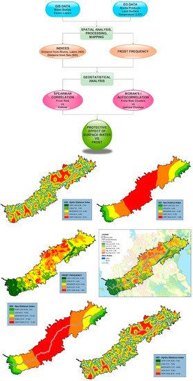
Figure 2. An example of integration of GIS and Earth Observation (EO) for frost monitoring [158].
Two criteria are often used for the recording of frost: the formation of ice crystals on surfaces (during field surveys) and meteorological measurements of air temperature [159]. As far as agriculture is concerned, frost can be described as a meteorological event when crops and other plants experience freezing injury due to occurrence of an air temperature less than 0 °C [151].
Meteorological measurements have high accuracy but have limited ability to describe the spatial heterogeneity of frost distribution [160]. Attempts to spatial interpolate air temperature measurements and frost often lead to unrepresentative spatial patterns, due to the low number and the irregular distribution of weather stations [161].
Nowadays, with the rapid technological and scientific development in Earth Observation (EO) technology, there is an upgraded potential in the study of the spatiotemporal distribution of frost. Especially in areas where temperature data are unavailable or expensive due to sparsity of meteorological stations or difficult access, remote sensing can be an important and valuable source of information [162]. Remote sensing data have been developed that provide ready to use products with information on night-time land surface temperature, through which frost can be recorded. The values of remotely sensed LST are determined from Planck’s Law using the emissivity of thermal infrared (TIR) bands. The quality of LST retrievals is affected by sensor characteristics, atmospheric conditions, variations in spectral emissivity, surface type heterogeneity, soil moisture, visualization geometry, and assumptions related to the split-window method [162].
A broadly used LST data source is the Moderate Resolution Imaging Spectrometer (MODIS) sensor, which has been providing information since 2000. The MODIS LST product (MOD11A1) has very high temporal resolution, with more than one revisit per day for some areas of the world, but its spatial resolution is course (1 km). The accuracy of the retrieved LST depends on the atmospheric and land surface conditions and is better than 1 °K in some cases [163].
An alternative source of night time LST is the Advanced Spaceborn Thermal Emission and Reflection Radiometer (ASTER) sensor. The accuracy of the ASTER LST product (AST-08–L.2) is calculated to be 0.3 °K and has a 90-m resolution for land areas, but its temporal resolution is lower, as its revisit time is at 16-day intervals [164].
A relatively recent thermal infrared sensor is the Landsat 8 Thermal Infrared Sensor (TIRS), with two adjacent thermal bands. Several approaches have been developed for the generation of LST from Landsat 8 data, such as the radiative transfer equation (RTE)-based method, the split-window (SW) algorithm and the single channel (SC) method. The highest estimated accuracy is accomplished with RTE, which is better than 1 °K [165].
Lastly, Sentinel-3 which has been developed by the European Space Agency and provides with LST data on a daily basis since 2017. The product SLSTR Level-2 LST product contains LST information with a spatial resolution of 1 km. The accuracy of the derived LST depends on atmosphere type and is estimated to be 0.8 °K for Polar Regions, 1.5 °K for mid-latitudes and 2 °K for equatorial latitudes [166].
In temperature fluctuation and frost monitoring studies, it is essential to have datasets with high spatial and temporal resolution. The limitations of the currently available EO data sets of either low temporal resolution, or low spatial resolution can be overcome by synthesizing high temporal resolution imagery with high spatial resolution imagery (Liu & Weng, 2012). The development of data fusion models such as Spatial and Temporal Adaptive Reflectance Fusion Model, has enabled the generation of ASTER-like daily land surface temperature with promising results [167][168][169][170].
5. Flood Monitoring
Natural disasters have significant impacts in many countries around the world, with a large number of deaths, damage to technical and infrastructure projects and population relocations. In addition, due to the significant impacts of climate change, these impacts are expected to increase in the coming years in many countries. Although technology and scientific knowledge have grown significantly today, natural disasters continue to have disastrous economic and environmental consequences, as well as many human casualties worldwide. The study and monitoring of these phenomena has been consistent in recent decades and has shown increasing trends [171]. In order to successfully monitor these phenomena and manage their impacts, it is very important to create hazard and risk maps for both the natural and the artificial environment [172][173].
Among the most dangerous and serious natural disasters, affecting more than 75 million people worldwide, are flood events [173]. In extreme flood events, it is important to quickly manage the magnitude of their impacts and land uses covered by water [174]. In this context, flood mapping and modeling are useful tools for monitoring, predicting, protecting, but also improving short and long term assistance to affected areas immediately after the event.
According to Lekkas [175], there are two types of floods, upstream and downstream. Upstream floods are observed in the higher parts of the drainage area and are generally the result of intense short-term rainfall in a small area. In contrast, downstream floods are caused by long-term storms that infiltrate the soil and cover a wide area. Most floods are the result of (i) the total amount and distribution of rainfall, (ii) the permeability of rock or soil, and (iii) the topography of an area. It has also been found that the distribution of land use, especially in small drainage basins, can significantly affect the size and frequency of floods. In addition, the risk of a flood in a watershed is determined by the following factors: land use, flood volume, intensity and frequency, elevation and duration of flood, season, weight of sediment deposited, and finally efficiency of monitoring, prediction, prevention, warning and emergency measures adaptation mechanisms [175].
New environmental challenges have put water resources monitoring and management at high academic and research interest. The local effects of climate change in recent decades, such as rising temperatures, decreasing rainfall (or increasing in other cases), desertification, etc., but also the occurrence of extreme phenomena such as storms, floods, landslides, and soil erosion threaten human life and infrastructure. The tendency to deal with this issue is rapidly increasing, due to the ever-increasing occurrence of such phenomena and the need for optimal monitoring and management, but also due to the technological boom that provides new tools and techniques. This constantly modifying and changing environmental regime has promoted the need for systematic research in related fields such as hydrology and/or hydraulics. Important goals of this endeavor are optimal methodological efficiency, comprehensive databases, and in particular state-of-the-art modeling developments, as well as understanding, monitoring and predicting an event or phenomenon of high importance nowadays. Modern geo-technologies (e.g., GIS and Remote Sensing) play a key role in this ongoing effort.
In the early 1980s, geographers argued that flood maps did not significantly influence people’s perception of floods and at the same time did not provide sufficient research planning. According to the Canadian Flood Disaster Reduction Program, although awareness of the effects of floods has increased among—after mapping—groups, it is not due to maps [176][177]. In an effort to improve this weakness many methods have been tried. Among these is the use of Remote Sensing (RS), which is not a new idea. In 1980, proving the previous argument, a research paper proposed the application of remote sensing for disaster monitoring and warning through various processes, such as flood mapping and assessment [178].
During the next decade, the use of Remote Sensing and GIS in flood monitoring and research became well established. Both passive and active sensors were used and tested, as can be understood by the two following references. Hubert-Moy et al. [179] suggested that the spatial analysis of Landsat Thematic Mapper (TM) is compatible for the study of floods in small catchments. The study also supported the fact that satellite image processing and flow analysis can simulate flood conditions even several days after the event’s peak, although the satellite’s repeatability is low. On the other hand, the usefulness of synthetic aperture radar (SAR) data was examined in a 1996 study. This study was able to compare satellite data on river floods with photographic recordings (taken from a small aircraft) aiming to demonstrate the accuracy of the SAR technique [180].
In 21st century GIS, Remote Sensing and other modern technologies play an important role in flood monitoring, analysis and mapping, but also in hydrological and/or hydraulic modeling, firmly established. Many scientists aimed to develop new ideas based on the above tools and techniques. Free software packages have been developed and distributed, huge global digital databases have been created and a multitude of research projects have been carried out. The evolution and revolution of hydrological and hydraulic modeling, as well as flood monitoring, analysis, and mapping, with modern technologies are flourishing, constantly finding new applications, satisfying ever-increasing demands—needs and inviting more and more young scientists to work in this field. The use of remote sensing data for monitoring and investigating floods and related phenomena (e.g., coastal impacts from sea level rise due to climate change) has increased rapidly in recent years. Various monitoring and research applications were based on RS data like LIDAR (Light Detection and Ranging) [181], RADARSAT SAR [182], NEXRAD III [183], EUMETSAT, SENTINEL [184][185][186], COSMO-SkyMed SAR [187], optical and microwave data US DMSP/Quikscat, RADARSAT, LANDSAT-5/7 (TM, ETM+), EOS-AM TERRA/MODIS, SRTM DEM and ASTER [188][189][190]. The continuous evolution and improvement of remote sensing data (coverage range, spatial resolution, data frequency, etc.) is expected to continuously increase their use and efficiency.
Furthermore, several scientists have attempted to exploit, or propose new, hydrological, hydraulic and other models along with remote sensing and GIS data and techniques, in order to investigate and monitor several issues directly or indirectly related to surface runoff and flooding [189][191][192][193][194][195]. At this point it is worth mentioning the development of the HYDROTEL hydrological model [196], the application of the hydrological model SLURP [197][198], the SWAT model (Soil and Water Assessment Tool) [199][200][201][202][203] and its evolution SWAT2000 [204], the HEC-HMS/RAS models [183][186][205][206][207][208][209][210][211], the naturally distributed WEP-L hydrological model [212], the MIKE11 model [213], spatially distributed hydrological model LIS-Flood model [214]. An example of the variety of applications, which combines hydrological and other models (e.g., SLEUTH) with Remote Sensing and GIS, is the study of urban sprawl [215][216].
The evolution of geographic–spatial analysis methods, and in particular of GIS, has been the forerunner and essence of change to the approach of flooding from purely mathematical–theoretical models and in situ research into a functional approach through spatial analysis, spatial models, geostatistics and other related methods, e.g., logistic regression, frequency analysis, etc. [185][217][218][219][220][221][222][223][224][225][226][227][228][229][230][231][232][233]. The next figure (Figure 3) provides such a context [230].
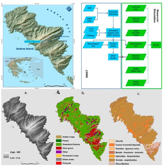
Figure 3. An example of GIS-based model for exploitation of floods via reservoirs ((a). DEM, (b). Land cover map, (c). Geology map) [230].
In general, the development of new technologies for rainfall–runoff modeling and flood monitoring, analysis, and forecasting, either in combination with GIS and Remote Sensing or autonomously, also involves the use of advanced methods such as Artificial Neural Networks (ANN), which are a highly evolving area of research [234][235], the application of fuzzy logic algorithms [236], SVM (Support Vector Machine) models [237].
The constant evolution of technology, as can be understood from the literature review, provides ever-more modern tools and techniques for the assessment and monitoring of natural disasters, and in particular floods. The development of new models (and the evolution of older ones), Geographic Information Systems, Remote Sensing, Applied Spatial Analysis, Geostatistics, etc., are some of the capabilities currently available to researchers, engineers, etc. to approach disastrous phenomena, such as floods. The need to apply these tools, to modernize existing methods, as well as to continually evolve and create new ones, is further enhanced by the effects of climate change and modern environmental, social, and economic requirements and needs.
6. Sea Level Rise Monitoring
According to the IPCC, (2018), global warming is likely to reach 1.5 °C between 2030 and 2052. Ablain et al. [238], explained in detail the importance of sea level rise, i.e., a measure of the increase in ocean volume, as a clear indicator of climate change and one of its main effects, by using data from European Space Agency (ESA) Earth Observation (EO) mission such as the ERS-1&2 and Envisat missions, the TOPEX/Poseidon, the Jason-1&2 and Geosat Follow-on (GFO) missions. Sea-level rise over the next century is expected to contribute significantly to physical changes along shorelines, enhancing coastal hazards particularly on low-gradient coastal zones, developing geodetic technologies and especially the Global Positioning System (GPS) [239][240]. Model-based projections of global mean sea level rise (relative to 1986–2005) suggest an indicative range of 0.26 to 0.77 m by 2100 for 1.5 °C of global warming [241].
Global warming is causing global mean sea level to rise mainly by the melting of glaciers and ice sheets resulting to the super induced addition of water into the ocean as well as by an increase of water body volume due to thermal expansion [242]. Relative sea level changes induced by variations for water in the oceans and land movements can be detected by tide gauges measurements, while EO satellite altimetry/gravimetry, as well as GPS satellites can be applied to measure absolute sea level changes at a global scale [243].
Tide gauges have been used since ancient times to record sea level variations but a well-developed network of tide gauges at almost 1000 locations around the globe, started to appear by the end of the nineteenth century. Moreover, the existence of altimeter satellites such as TOPEX/POSEIDO creates the opportunity for even better measures [244][245][246]. Human activities are estimated to have caused global mean sea level rise of about 21–24 cm since 1880 and even though there is a network of tide gauges provides valuable information about sea level changes from a few seconds to centuries [247][248][249], these observations suffer from several limitations, i.e., their geographic distribution which is poor in open oceans or the southern hemisphere, the availability of records which is not contemporary for all stations and the effect of vertical land movements which is the one of the main difficulties to interpret tide gauge measurements [244][250].
On the other hand, satellite altimetry together with SAR altimetry is described by Cipollini et al. [251] as one of the workhorses of open-ocean operational oceanography and global sea level monitoring, providing for more than 28 years valuable data sea level date with accuracies of the order of just a few cm even for the most remote areas of the oceans. Major support has been provided to the international scientific community by several space agencies such as the National Aeronautics and Space Administration (NASA), the European Space Agency (ESA) and the Centre National d’Etudes Spatiales (CNES) in research and development of innovative techniques for coastal altimetry.
According to Ablain et al. [238] satellite altimetry data fit well with tide gauge measurements, however it is of great importance to be able to link the satellite altimeter measurements of sea level rise with the tide gauge measurements, by bridging the open-ocean measurements with those in close proximity to the coast in order to meet the scientific needs for better data resolution.
GIS has proved that when it is integrated with remote sensing data and tide gauge measurements, it has the potential to act as an important tool in monitoring the environmental and socio-economic effects of sea-level rise. GIS is increasingly used as a support tool in sea-level rise monitoring, as it allows homogenization and integration of all the available data into a geodatabase, in order to access information, perform spatial and geostatistical analysis and it has a strong potential to combine a broad range of complex variables and data in varying formats and to integrate physical, ecological, socioeconomic, and hazards information. Furthermore, owing to its numerous advantages such as editing and data automation, visualization, mapping and map-based tasks, spatial consultation, spatial analysis, and geostatistical analysis and its flexibility, GIS can be used in further planning applications and future scenarios. Over the years GIS has shown great potential in its application and problem-solving capabilities and a great number of researchers have applied GIS-based methodologies to study sea level rise globally and regionally.
This entry is adapted from the peer-reviewed paper 10.3390/ijgi10020094
References
- Karavitis, C. Drought Management Strategies for Urban Water Supplies: The Case of Metropolitan Athens. Ph.D. Thesis, Department of Civil Engineering, Colorado State University, Fort Collins, CO, USA, 1992.
- Kalabokidis, K.D.; Karavitis, C.; Vasilakos, C. Automated fire and flood danger assessment system. In Proceedings of the International Workshop on Forest Fires in the Wildland-Urban Interface and Rural Areas in Europe; MAICH: Crete, Greece, 2004; pp. 143–153.
- Kalabokidis, K.; Kallos, G.; Karavitis, C.; Caballero, D.; Tettelaar, P.; Llorens, J.; Vasilakos, C. Automated fire and flood hazard protection system. In Proceedings of the 5th International Workshop on Remote Sensing and GIS Applications to Forest Fire Management: Fire Effects Assessment, Zaragoza, Spain, 16–18 June 2005; Universidad de Zaragoza: Zaragoza, Spain, 2005; pp. 167–172.
- Tsesmelis, D.E.; Oikonomou, P.D.; Vasilakou, C.G.; Skondras, N.A.; Fassouli, V.; Alexandris, S.G.; Grigg, N.S.; Karavitis, C.A. Assessing structural uncertainty caused by different weighting methods on the Standardized Drought Vulnerability Index (SDVI). Stoch. Environ. Res. Risk Assess. 2019, 33, 515–533.
- Karavitis, C.A.; Tsesmelis, D.E.; Skondras, N.A.; Stamatakos, D.; Alexandris, S.; Fassouli, V.; Vasilakou, C.G.; Oikonomou, P.D.; Gregorič, G.; Grigg, N.S.; et al. Linking drought characteristics to impacts on a spatial and temporal scale. Water Policy 2014, 16, 1172–1197.
- Wilhite, D.A. Chapter 1 Drought as a Natural Hazard: Concepts and Definitions; Drought Mitigation Center Faculty Publications: Lincoln, NE, USA, 2000.
- Sonmez, K.; Komuscu, A.U.; Erkan, A.; Turgu, E. An Analysis of Spatial and Temporal Dimension of Drought Vulnerability in Turkey Using the Standardized Precipitation Index. Nat. Hazards 2005, 35, 243–264.
- Grigg, N.S.; Vlachos, E.C. Drought Water Management; International School for Water Resources, Department of Civil Engineering, Colorado State University: Fort Collins, CO, USA, 1990.
- Karavitis, C.A. Drought and urban water supplies: The case of metropolitan Athens. Water Policy 1998, 1, 505–524.
- Yevjevich, V.; Da Cunha, L.; Vlachos, E. Coping with Droughts; Water Resources Publications: Littleton, CO, USA, 1983.
- Karavitis, C.A. Decision Support Systems for Drought Management Strategies in Metropolitan Athens. Water Int. 1999, 24, 10–21.
- Bordi, I.; Fraedrich, K.; Petitta, M.; Sutera, A. Large-Scale Assessment of Drought Variability Based on NCEP/NCAR and ERA-40 Re-Analyses. Water Resour. Manag. 2006, 20, 899–915.
- Mishra, A.K.; Singh, V.P. A review of drought concepts. J. Hydrol. 2010, 391, 202–216.
- Oikonomou, P.D.; Tsesmelis, D.E.; Waskom, R.M.; Grigg, N.S.; Karavitis, C.A. Enhancing the Standardized Drought Vulnerability Index by Integrating Spatiotemporal Information from Satellite and In Situ Data. J. Hydrol. 2019, 569, 265–277.
- Adger, W.N. Vulnerability. Glob. Environ. Chang. 2006, 16, 268–281.
- Horton, G.; Hanna, L.; Kelly, B. Drought, drying and climate change: Emerging health issues for ageing Australians in rural areas. Australas. J. Ageing 2010, 29, 2–7.
- Wilhite, D.A.; Sivakumar, M.V.K.; Pulwarty, R. Managing drought risk in a changing climate: The role of national drought policy. Weather Clim. Extrem. 2014, 3, 4–13.
- Ciais, P.; Reichstein, M.; Viovy, N.; Granier, A.; Ogée, J.; Allard, V.; Aubinet, M.; Buchmann, N.; Bernhofer, C.; Carrara, A.; et al. Europe-wide reduction in primary productivity caused by the heat and drought in 2003. Nature 2005, 437, 529–533.
- Oikonomou, P.D.; Karavitis, C.A.; Tsesmelis, D.E.; Kolokytha, E.; Maia, R. Drought Characteristics Assessment in Europe over the Past 50 Years. Water Resources Management. 2020, 34, 4757–4772.
- Tsesmelis, D.E. Development, Implementation and Evaluation of Drought and Desertification Risk Indicators for the Integrated Management of Water Resources. Ph.D. Thesis, Department of Natural Resources Management & Agricultural Engineering, Agricultural University of Athens, Athens, Greece, 2017.
- Karavitis, C.A.; Alexandris, S.; Tsesmelis, D.E.; Athanasopoulos, G. Application of the Standardized Precipitation Index (SPI) in Greece. Water 2011, 3, 787–805.
- Karavitis, C.A.; Chortaria, C.; Alexandris, S.; Vasilakou, C.G.; Tsesmelis, D.E. Development of the standardised precipitation index for Greece. Urban. Water J. 2012, 9, 401–417.
- Pedro-Monzonís, M.; Ferrer, J.; Solera, A.; Estrela, T.; Paredes-Arquiola, J. Key issues for determining the exploitable water resources in a Mediterranean river basin. Sci. Total Environ. 2015, 503–504, 319–328.
- Pedro-Monzonís, M.; Solera, A.; Ferrer, J.; Estrela, T.; Paredes-Arquiola, J. A review of water scarcity and drought indexes in water resources planning and management. J. Hydrol. 2015, 527, 482–493.
- Loucks, D.P. Sustainable Water Resources Management. Water Int. 2000, 25, 3–10.
- Wilhite, D.A.; Hayes, M.J.; Knutson, C.; Smith, K.H. Planning for drought: Moving from crisis to risk management. JAWRA J. Am. Water Resour. Assoc. 2000, 36, 697–710.
- Kampragou, E.; Apostolaki, S.; Manoli, E.; Froebrich, J.; Assimacopoulos, D. Towards the harmonization of water-related policies for managing drought risks across the EU. Environ. Sci. Policy 2011, 14, 815–824.
- Skondras, N.A.; Karavitis, C.A.; Gkotsis, I.I.; Scott, P.J.B.; Kaly, U.L.; Alexandris, S.G. Application and assessment of the Environmental Vulnerability Index in Greece. Ecol. Indic. 2011, 11, 1699–1706.
- Skondras, N. Decision Making in Water Resources Management: Development of a Composite Indicator for the Assessment of the Social-Environmental Systems in Terms Resilience and Vulnerability to Water Scarcity and Water Stress. Ph.D. Thesis, Department of Natural Resources Management and Agricultural Engineering, Agricultural University of Athens, Athens, Greece, 2015.
- Cancelliere, A.; Mauro, G.D.; Bonaccorso, B.; Rossi, G. Drought forecasting using the Standardized Precipitation Index. Water Resour. Manag. 2007, 21, 801–819.
- Priscoli, J.D. Keynote Address: Clothing the IWRM Emperor by Using Collaborative Modeling for Decision Support. JAWRA J. Am. Water Resour. Assoc. 2013, 49, 609–613.
- Salas, J.D.; Fu, C.; Cancelliere, A.; Dustin, D.; Bode, D.; Pineda, A.; Vincent, E. Characterizing the Severity and Risk of Drought in the Poudre River, Colorado. J. Water Resour. Plan. Manag. 2005, 131, 383–393.
- Vlachos, E. Prologue: Water peace and conflict management. Water Int. 1990, 15, 185–188.
- Vlachos, E.; Braga, B. The challenge of urban water management. In Proceedings of the Frontiers in Urban Water Management: Deadlock or Hope; IWA Publishing: London, UK, 2001; pp. 1–36.
- Grigg, N.S. Water Resources Management. In Water Encyclopedia; John Wiley & Sons, Inc.: Hoboken, NJ, USA, 1996.
- Tsesmelis, D.E.; Karavitis, C.A.; Oikonomou, P.D.; Alexandris, S.; Kosmas, C. Assessment of the Vulnerability to Drought and Desertification Characteristics Using the Standardized Drought Vulnerability Index (SDVI) and the Environmentally Sensitive Areas Index (ESAI). Resources 2019, 8, 6.
- Swathandran, S.; Aslam, M.A.M. Assessing the role of SWIR band in detecting agricultural crop stress: A case study of Raichur district, Karnataka, India. Environ. Monit. Assess. 2019, 191, 442.
- Vlachos, E.C. Drought Management Interfaces; ASCE: Las Vegas, NE, USA, 1982; p. 15.
- AghaKouchak, A.; Feldman, D.; Hoerling, M.; Huxman, T.; Lund, J. Water and climate: Recognize anthropogenic drought. Nat. News 2015, 524, 409.
- Tsakiris, G.; Pangalou, D.; Vangelis, H. Regional Drought Assessment Based on the Reconnaissance Drought Index (RDI). Water Resour. Manag. 2007, 21, 821–833.
- Vangelis, H.; Tigkas, D.; Tsakiris, G. The effect of PET method on Reconnaissance Drought Index (RDI) calculation. J. Arid Environ. 2013, 88, 130–140.
- Fassouli, V. Development, Implementation and Assessment of a Composite Index for the Identification and Classification of Drought and Creation of the Corresponding Decision Support System. Ph.D. Thesis, Department of Natural Resources Management & Agricultural Engineering, Agricultural University of Athens, Athens, Greece, 2017.
- Rossi, G.; Benedini, M.; Tsakiris, G.; Giakoumakis, S. On regional drought estimation and analysis. Water Resour. Manag. 1992, 6, 249–277.
- Pimentel, D. Soil erosion: A food and environmental threat. Environ. Dev. Sustain. 2006, 8, 119–137.
- Lal, R. Soil erosion and the global carbon budget. Environ. Int. 2003, 29, 437–450.
- Milliman, J.D.; Syvitski, J.P.M. Geomorphic/tectonic control of sediment discharge to the ocean: The importance of small mountainous rivers. J. Geol. 1992, 100, 525–544.
- Walling, D.E.; Webb, B.W. Erosion and sediment yield: A global overview. In Erosion and Sediment Yield: Global and Regional Perspectives Proceedings of the Exeter Symposium; Walling, D.E., Webb, B.W., Eds.; IAHS Publication No. 236; ISI: Exeter, UK, 1996; pp. 3–19.
- Polykretis, C.; Alexakis, D.D.; Grillakis, M.G.; Manoudakis, S. Assessment of Intra-Annual and Inter-Annual Variabilities of Soil Erosion in Crete Island (Greece) by Incorporating the Dynamic “Nature” of R and C-Factors in RUSLE Modeling. Remote Sens. 2020, 12, 2439.
- Lai, R. Soil degradation by erosion. Land Degrad. Dev. 2001, 12, 519–539.
- Xu, L.; Xu, X.; Meng, X. Risk assessment of soil erosion in different rainfall scenarios by RUSLE model coupled with Information Diffusion Model: A case study of Bohai Rim, China. Catena 2013, 100, 74–82.
- Nearing, M.A.; Pruski, F.F.; O’neal, M.R. Expected climate change impacts on soil erosion rates: A review. J. Soil Water Conserv. 2004, 59, 43–50.
- Ganasri, B.P.; Ramesh, H. Assessment of soil erosion by RUSLE model using remote sensing and GIS-A case study of Nethravathi Basin. Geosci. Front. 2016, 7, 953–961.
- Oldeman, L.R.; Van Engelen, V.W.P.; Pulles, J.H.M. The extent of human induced soil degradation. In Annex 5 of World Man of the Status of Human-Induced Soil Degradation: An. Explanatory Note, 2nd ed.; Oldeman, L.R., Hakkeling, R.T.A., Sombroek, W.G., Eds.; International Soil Reference and Information Center: Wageningen, The Netherlands, 1990.
- Fistikoglu, O.; Harmancioglu, N.B. Integration of GIS with USLE in assessment of soil erosion. Water Resour. Manag. 2002, 16, 447–467.
- Kothyari, U.C. Erosion and sediment problems in India. In Proceedings of the Exeter Symposium on Erosion and Sediment Yield: Global and Regional Perspectives; IAHS Publication No. 236; ISI: Exeter, UK, 1996; pp. 531–540.
- Jha, M.K.; Paudel, R.C. Erosion predictions by empirical models in a mountainous watershed in Nepal. J. Spat. Hydrol. 2010, 10, 89–102.
- Wischmeier, W.H.; Smith, D.D. Predicting Rainfall Erosion Losses: A Guide to Conservation Planning; Agriculture Handbook No. 537; USDA: Washington, DC, USA, 1978.
- Karydas, C.G.; Panagos, P.; Gitas, I.Z. A classification of water erosion models according to their geospatial characteristics. Int. J. Digit. Earth 2014, 7, 229–250.
- Zhang, Z.-H.; Gang, H.U.; Jian, N.I. Effects of Topographical and Edaphic Factors on the Distribution of Plant Communities in Two Subtropical Karst Forests, Southwestern China. J. Mt. Sci. 2013, 10, 95–104.
- Lee, G.S.; Lee, K.H. Scaling effect for estimating soil loss in the RUSLE model using remotely sensed geospatial data in Korea. J. Hydrol. Earth Syst. Sci. 2006, 3, 135–157.
- Remortel Van, R.; Hamilton, M.; Hickey, R. Estimating the LS factor for RUSLE through iterative slope length processing of digital elevation data. Cartography 2001, 30, 27–35.
- Eckelmann, W.; Baritz, R.; Bialousz, S.; Bielek, P.; Carré, F.; Hrušková, B.; Jones, R.J.; Kibblewhite, M.; Kozak, J.; Le Bas, C.; et al. Common Criteria for Risk Area Identification According to Soil Threats; Office for Official Publications of the European Communities: Brussels, Belgium, 2006.
- Van Beek, C.L.; Tóth, T.; Hagyó, A.; Tóth, G.; Recatalá Boix, L.; Añó Vidal, C.; Malet, J.P.; Maquaire, O.; Van den Akker, J.J.H.; Van der Zee, S.; et al. The need for harmonizing methodologies for assessing soil threats in Europe. Soil Use Manag. 2010, 26, 299–309.
- Rozos, D.; Skilodimou, H.D.; Loupasakis, C.; Bathrellos, G.D. Application of the revised universal soil loss equation model on landslide prevention. An example from N. Euboea (Evia) Island, Greece. Environ. Earth Sci. 2013, 70, 3255–3266.
- Fernandez, P.; Delgado, E.; Lopez-Alonso, M.; Poyatos, J.M. GIS environmental information analysis of the Darro River basin as the key for the management and hydrological forest restoration. Sci. Total Environ. 2018, 613, 1154–1164.
- De Jong, S.M. Applications of reflective remote sensing for land degradation studies in a Mediterranean environment. Ph.D. Thesis, Utrecht University, Utrecht, The Netherlands, 1994.
- De Vente, J.; Poesen, J. Predicting soil erosion and sediment yield at the basin scale: Scale issues and semi-quantitative models. Earth Sci. Rev. 2005, 71, 95–125.
- Giordano, A.; Bonfils, P.; Briggs, D.J.; de Sequeira, E.M.; de Laburu, C.R.; Yassoglou, N. The methodological approach to soil erosion and important land resources evaluation of the European Community. Soil Technol. 1991, 4, 65–77.
- Stathopoulos, N.; Lykoudi, E.; Vasileiou, E.; Rozos, D.; Dimitrakopoulos, D. Erosion Vulnerability Assessment of Sperchios River Basin, in East Central Greece—A GIS Based Analysis. Open J. Geol. 2017, 7, 621–646.
- Gitas, Ι.Z.; Douros, K.; Minakou, C.; Silleos, G.N.; Karydas, C.G. Multi-temporal soil erosion risk assessment in N. Chalkidiki using a modified USLE raster model. EARSeL eProceedings 2009, 8, 40–52.
- Fernandez, C.; Wu, J.Q.; McCool, D.Q.; Stockle, C.O. Estimating water erosion and sediment yield with GIS, RUSLE and SEDD. J. Soil Water Conserv. 2003, 58, 128–136.
- Alemayehu, F.; Taha, N.; Nyssen, J.; Girma, A.; Zenebe, A.; Behailu, M.; Deckers, S.; Poesen, J. The impacts of watershed management on land use and land cover dynamics in Eastern Tigray (Ethiopia). Resour. Conserv. Recycl. 2009, 53, 192–198.
- Rahman, M.R.; Shi, Z.H.; Chongfa, C. Soil erosion hazard evaluation—An integrated use of remote sensing, GIS and statistical approaches with biophysical parameters towards management strategies. Ecol. Model. 2009, 220, 1724–1734.
- Alexakis, D.D.; Hadjimitsis, D.G.; Agapiou, A. Integrated use of remote sensing, GIS and precipitation data for the assessment of soil erosion rate in the catchment area of “Yialias” in Cyprus. Atmos. Res. 2013, 131, 108–124.
- Künzer, C.; Ottinger, M.; Liu, G.; Sun, B.; Baumhauer, R.; Dech, S. Earth observation-based coastal zone monitoring of the Yellow River Delta: Dynamics in China’s second largest oil producing region over four decades. Appl. Geogr. 2014, 55, 92–107.
- Alexandridis, T.K.; Sotiropoulou, A.M.; Bilas, G.; Karapetsas, N.; Silleos, N.G. The Effects of Seasonality in Estimating the C-Factor of Soil Erosion Studies. Land Degrad. Dev. 2015, 26, 596–603.
- Ghosh, M.K.; Kumar, L.; Roy, C. Monitoring the coastline change of Hatiya Island in Bangladesh using remote sensing techniques. ISPRS J. Photogramm. Remote Sens. 2015, 101, 137–144.
- AbdelRahman, M.A.; Natarajan, A.; Hegde, R. Assessment of land suitability and capability by integrating remote sensing and GIS for agriculture in Chamarajanagar district, Karnataka, India. Egypt. J. Remote Sens. Space Sci. 2016, 19, 125–141.
- Neugirg, F.; Stark, M.; Kaiser, A.; Vlacilova, M.; Della Seta, M.; Vergari, F.; Schmidt, J.; Becht, M.; Haas, F. Erosion processes in calanchi in the Upper Orcia Valley, Southern Tuscany, Italy based on multitemporal high-resolution terrestrial LiDAR and UAV surveys. Geomorphology 2016, 269, 8–22.
- Rayegani, B.; Barati, S.; Sohrabi, T.A.; Sonboli, B. Remotely sensed data capacities to assess soil degradation. Egypt. J. Remote Sens. Space Sci. 2016, 19, 207–222.
- Dewan, A.; Corner, R.; Saleem, A.; Rahman, M.M.; Haider, M.R.; Rahman, M.M.; Sarker, M.H. Assessing channel changes of the Ganges-Padma River system in Bangladesh using Landsat and hydrological data. Geomorphology 2017, 276, 257–279.
- Chappell, A.; Webb, N.P.; Guerschman, J.P.; Thomas, D.T.; Mata, G.; Handcock, R.N.; Leys, J.F.; Butler, H.J. Improving ground cover monitoring for wind erosion assessment using MODIS BRDF parameters. Remote Sens. Environ. 2018, 204, 756–768.
- Nigel, R.; Rughooputh, S. Mapping of monthly soil erosion risk of mainland Mauritius and its aggregation with delineated basins. Geomorphology 2010, 114, 101–114.
- Jain, M.K.; Das, D. Estimation of sediment yield and areas of soil erosion and deposition for watershed prioritization using GIS and remote sensing. Water Resour. Manag. 2010, 24, 2091–2112.
- Chou, W.C. Modelling watershed scale soil loss prediction and sediment yield estimation. Water Resour. Manag. 2010, 24, 2075–2090.
- Hui, L.; Xiaoling, C.; Lim, K.J.; Xiaobin, C.; Sagong, M. Assessment of soil erosion and sediment yield in Liao watershed, Jiangxi Province, China, Using USLE, GIS, and RS. J. Earth Sci. 2010, 21, 941–953.
- Ouyang, W.; Hao, F.; Skidmore, A.K.; Toxopeus, A.G. Soil erosion and sediment yield and their relationships with vegetation cover in upper stream of the Yellow River. Sci. Total Environ. 2010, 409, 396–403.
- Demirci, A.; Karaburun, A. Estimation of soil erosion using RUSLE in a GIS framework: A case study in the Buyukcekmece Lake watershed, northwest Turkey. Environ. Earth Sci. 2012, 66, 903–913.
- Mhangara, P.; Kakembo, V.; Lim, K.J. Soil erosion risk assessment of the Keiskamma catchment, South Africa using GIS and remote sensing. Environ. Earth Sci. 2012, 65, 2087–2102.
- Pradhan, B.; Chaudhari, A.; Adinarayana, J.; Buchroithner, M.F. Soil erosion assessment and its correlation with landslide events using remote sensing data and GIS: A case study at Penang Island, Malaysia. Environ. Monit. Assess. 2012, 184, 715–727.
- Prasannakumar, V.; Vijith, H.; Abinod, S.; Geetha, N. Estimation of soil erosion risk within a small mountainous sub-watershed in Kerala, India, using Revised Universal Soil Loss Equation (RUSLE) and geo-information technology. Geosci. Front. 2012, 3, 209–215.
- Ranzi, R.; Le, T.H.; Rulli, M.C. A RUSLE approach to model suspended sediment load in the Lo river (Vietnam): Effects of reservoirs and land use changes. J. Hydrol. 2012, 422, 17–29.
- Esteves, T.C.J.; Kirkby, M.J.; Shakesby, R.A.; Ferreira, A.J.D.; Soares, J.A.A.; Irvine, B.J.; Ferreira, C.S.S.; Coelho, C.O.A.; Bento, C.P.M.; Carreiras, M.A. Mitigating land degradation caused by wildfire: Application of the PESERA model to fire-affected sites in central Portugal. Geoderma 2012, 191, 40–50.
- Chatterjee, S.; Krishna, A.P.; Sharma, A.P. Geospatial assessment of soil erosion vulnerability at watershed level in some sections of the Upper Subarnarekha river basin, Jharkhand, India. Environ. Earth Sci. 2014, 71, 357–374.
- Sun, W.; Shao, Q.; Liu, J.; Zhai, J. Assessing the effects of land use and topography on soil erosion on the Loess Plateau in China. Catena 2014, 121, 151–163.
- Cilek, A.; Berberoglu, S.; Kirkby, M.; Irvine, B.; Donmez, C.; Erdogan, M.A. Erosion modelling in a Mediterranean subcatchment under climate change scenarios using Pan-European Soil Erosion Risk Assessment (PESERA). Int. Arch. Photogramm. Remote Sens. Spat. Inf. Sci. 2015, 40, 359.
- Aiello, A.; Adamo, M.; Canora, F. Remote sensing and GIS to assess soil erosion with RUSLE3D and USPED at river basin scale in southern Italy. Catena 2015, 131, 174–185.
- Gaubi, I.; Chaabani, A.; Mammou, A.B.; Hamza, M.H. A GIS-based soil erosion prediction using the Revised Universal Soil Loss Equation (RUSLE) (Lebna watershed, Cap Bon, Tunisia). Nat. Hazards 2017, 86, 219–239.
- Bera, A. Estimation of soil loss by USLE model using GIS and remote sensing techniques: A case study of Muhuri River Basin, Tripura, India. Eurasian J. Soil Sci. 2017, 6, 206.
- Bouguerra, H.; Bouanani, A.; Khanchoul, K.; Derdous, O.; Tachi, S.E. Mapping erosion prone areas in the Bouhamdane watershed (Algeria) using the Revised Universal Soil Loss Equation through GIS. J. Water Land Dev. 2017, 32, 13–23.
- Karydas, C.G.; Panagos, P. The G2 erosion model: An algorithm for month-time step assessments. Environ. Res. 2018, 161, 256–267.
- Leh, M.; Bajwa, S.; Chaubey, I. Impact of land use change on erosion risk: An integrated remote sensing, geographic information system and modeling methodology. Land Degrad. Dev. 2013, 24, 409–421.
- Park, S.; Oh, C.; Jeon, S.; Jung, H.; Choi, C. Soil erosion risk in Korean watersheds, assessed using the revised universal soil loss equation. J. Hydrol. 2011, 399, 263–273.
- Chowdary, V.M.; Chakraborthy, D.; Jeyaram, A.; Murthy, Y.K.; Sharma, J.R.; Dadhwal, V.K. Multi-criteria decision making approach for watershed prioritization using analytic hierarchy process technique and GIS. Water Resour. Manag. 2013, 27, 3555–3571.
- Badar, B.; Romshoo, S.A.; Khan, M.A. Integrating biophysical and socioeconomic information for prioritizing watersheds in a Kashmir Himalayan lake: A remote sensing and GIS approach. Environ. Monit. Assess. 2013, 185, 6419–6445.
- Mello, C.D.; Viola, M.R.; Beskow, S.; Norton, L.D. Multivariate models for annual rainfall erosivity in Brazil. Geoderma 2013, 202, 88–102.
- Thomas, J.; Joseph, S.; Thrivikramji, K.P. Assessment of soil erosion in a tropical mountain river basin of the southern Western Ghats, India using RUSLE and GIS. Geosci. Front. 2018, 9, 893–906.
- Macedo, D.R.; Hughes, R.M.; Kaufmann, P.R.; Callisto, M. Development and validation of an environmental fragility index (EFI) for the neotropical savannah biome. Sci. Total Environ. 2018, 635, 1267–1279.
- Tetzlaff, B.; Friedrich, K.; Vorderbrügge, T.; Vereecken, H.; Wendland, F. Distributed modelling of mean annual soil erosion and sediment delivery rates to surface waters. Catena 2013, 102, 13–20.
- Shi, Z.H.; Cai, C.F.; Ding, S.W.; Wang, T.W.; Chow, T.L. Soil conservation planning at the small watershed level using RUSLE with GIS: A case study in the Three Gorge Area of China. Catena 2004, 55, 33–48.
- Şahin, Ş.; Kurum, E. Erosion risk analysis by GIS in environmental impact assessments: A case study—Seyhan Köprü Dam construction. J. Environ. Manag. 2002, 66, 239–247.
- Millward, A.A.; Mersey, J.E. Conservation strategies for effective land management of protected areas using an erosion prediction information system (EPIS). J. Environ. Manag. 2001, 61, 329–343.
- Aguirre, J.A.M.; Sánchez, J.C.R. Caracterización de las cuencas hidrográficas, objeto de restauración higrológico-forestal, mediante modelos hidrológicos. Ing. Del Agua 1994, 1, 2.
- Tabesh, M.; Saber, H. A prioritization model for rehabilitation of water distribution networks using GIS. Water Resour. Manag. 2012, 26, 225–241.
- Tang, Z.; Li, X.; Zhao, N.; Li, R.; Harvey, E.F. Developing a restorable wetland index for rainwater basin wetlands in south-central Nebraska: A multi-criteria spatial analysis. Wetlands 2012, 32, 975–984.
- Nekhay, O.; Arriaza, M.; Boerboom, L. Evaluation of soil erosion risk using Analytic Network Process and GIS: A case study from Spanish mountain olive plantations. J. Environ. Manag. 2009, 90, 3091–3104.
- De Paz, J.M.; Sánchez, J.; Visconti, F. Combined use of GIS and environmental indicators for assessment of chemical, physical and biological soil degradation in a Spanish Mediterranean region. J. Environ. Manag. 2006, 79, 150–162.
- Liu, C.; Frasier, P.; Kumar, L.; Macgregor, C. Catchmentwide wetland assessment and prioritization using the multi-criteria decision making method TOPIS. Environ. Manag. 2006, 38, 316–326.
- Metternicht, G.; Gonzalez, S. FUERO: Foundations of a fuzzy exploratory model for soil erosion hazard prediction. Environ. Model. Softw. 2005, 20, 715–728.
- Navas, A.; Machín, J.; Soto, J. Assessing soil erosion in a Pyrenean mountain catchment using GIS and fallout 137Cs. Agric. Ecosyst. Environ. 2005, 105, 493–506.
- Finlayson, D.P.; Montgomery, D.R. Modelling large-scale fluvial erosion in geographic information systems. Geomorphology 2003, 53, 147–164.
- Chowdhury, A.; Jha, M.K.; Chowdary, V.M.; Mal, B.C. Integrated remote sensing and GIS-based approach for assessing groundwater potential in West Medinipur district, West Bengal, India. Int. J. Remote Sens. 2009, 30, 231–250.
- Magesh, N.S.; Chandrasekar, N.; Soundranayagam, J.P. Delineation of groundwater potential zones in Theni district, Tamil Nadu, using remote sensing, GIS and MIF techniques. Geosci. Front. 2012, 3, 189–196.
- Babiker, I.S.; Mohamed, M.A.; Hiyama, T. Assessing groundwater quality using GIS. Water Resour. Manag. 2007, 21, 699–715.
- Mukherjee, S.; Veer, V.; Tyagi, S.K.; Sharma, V. Sedimentation study of Hirakud reservoir through remote sensing techniques. J. Spat. Hydrol. 2007, 7, 1.
- Saraf, A.K.; Choudhury, P.R. Integrated remote sensing and GIS for groundwater exploration and identification of artificial recharge sites. Int. J. Remote Sens. 1998, 19, 1825–1841.
- Babiker, I.S.; Mohamed, M.A.; Terao, H.; Kato, K.; Ohta, K. Assessment of groundwater contamination by nitrate leaching from intensive vegetable cultivation using geographical information system. Environ. Int. 2004, 29, 1009–1017.
- Shetkar, R.V.; Mahesha, A. Tropical, seasonal river basin development: Hydrogeological analysis. J. Hydrol. Eng. 2004, 16, 280–291.
- Sener, E.; Davraz, A.; Ozcelik, M. An integration of GIS and remote sensing in groundwater investigations: A case study in Burdur, Turkey. Hydrogeol. J. 2005, 13, 826–834.
- Engman, E.T.; Gurney, R.J. Remote Sensing in Hydrology; Chapman and Hall: London, UK, 1991.
- Jha, M.K.; Chowdhury, A.; Chowdary, V.M.; Peiffer, S. Groundwater management and development by integrated remote sensing and geographic information systems: Prospects and constraints. Water Resour. Manag. 2007, 21, 427–467.
- Todd, D.K. Groundwater Hydrogeology, 2nd ed.; John Wiley & Son: New York, NY, USA, 1980.
- Jha, M.K.; Peiffer, S. Applications of Remote Sensing and GIS Technologies in Groundwater Hydrology: Past, Present and Future; BayCEER: Bayreuth, Germany, 2006; p. 201.
- Tiwari, A.; Rai, B. Hydromorphogeological mapping for groundwater prospecting using landsat-MSS images—a case study of part of Dhanbad District, Bihar. J. Indian Soc. Remote Sens. 1996, 24, 281–285.
- Das, S.; Behera, S.C.; Kar, A.; Narendra, P.; Guha, S. Hydrogeomorphological mapping in ground water exploration using remotely sensed data—a case study in keonjhar district, orissa. J. Indian Soc. Remote Sens. 1997, 25, 247–259.
- Thomas, A.; Sharma, P.K.; Sharma, M.K.; Sood, A. Hydrogeomorphological mapping in assessing ground water by using remote sensing data—A case study in lehra gaga block, sangrur district, Punjab. J. Indian Soc. Remote Sens. 1999, 27, 31.
- Harinarayanan, P.; Gopalakrishna, G.S.; Balasubramanian, A. Remote sensing data for groundwater development and management in Keralapura watersheds of Cauvery Basin, Karnataka, India. Indian Mineral. 2000, 34, 11–17.
- Muralidhar, M.; Raju, K.R.K.; Raju, K.S.V.P.; Prasad, J.R. Remote sensing applications for the evaluation of water resources in rainfed area, Warangal district, Andhra Pradesh. Indian Miner. 2000, 34, 33–40.
- Chowdhury, A.; Jha, M.K.; Chowdary, V.M. Delineation of groundwater recharge zones and identification of artificial recharge sites in West Medinipur district, West Bengal, using RS, GIS and MCDM techniques. Environ. Earth Sci. 2010, 59, 1209.
- Stafford, D.B. Civil Engineering Applications of Remote Sensing and Geographic Information Systems; ASCE: Reston, VA, USA, 1991.
- Goodchild, M.F. The state of GIS for environmental problem-solving. In Environmental Modeling with GIS; IntechOpen: London, UK, 1993; pp. 8–15.
- Chopra, R.; Sharma, P.K. Landform analysis and ground water potential in the Bist Doab area, Punjab, India. Int. J. Remote Sens. 1993, 14, 3221–3229.
- Sander, P. Water-well siting in hard-rock areas: Identifying promising targets using a probabilistic approach. Hydrogeol. J. 1997, 5, 32–43.
- Teeuw, R.M. Groundwater exploration using remote sensing and a low-cost geographical information system. Hydrogeol. J. 1995, 3, 21–30.
- Dar, I.A.; Sankar, K.; Dar, M.A. Deciphering groundwater potential zones in hard rock terrain using geospatial technology. Environ. Monit. Assess. 2011, 173, 597–610.
- Kumar, S.K.; Chandrasekar, N.; Seralathan, P.; Godson, P.S.; Magesh, N.S. Hydrogeochemical study of shallow carbonate aquifers, Rameswaram Island, India. Environ. Monit. Assess. 2012, 184, 4127–4138.
- Jankowski, P. Integrating geographical information systems and multiple criteria decision-making methods. Int. J. Geogr. Inf. Syst. 1995, 9, 251–273.
- Solomon, S.; Quiel, F. Groundwater study using remote sensing and geographic information systems (GIS) in the central highlands of Eritrea. Hydrogeol. J. 2006, 14, 229–741.
- Prasad, R.K.; Mondal, N.C.; Banerjee, P.; Nandakumar, M.V.; Singh, V.S. Deciphering potential groundwater zone in hard rock through the application of GIS. Environ. Geol. 2008, 55, 467–475.
- Gustafsson, P. High Resolution Satellite Imagery and GIS as a Dynamic Tool in Groundwater Exploration in a Semi-arid Area; IAHS Publication: Wallingford, UK, 1993.
- Snyder, R.L.; Melo-Abreu, J.D. Frost Protection: Fundamentals, Practice and Economics; Food and Agriculture Organization of the United Nations: Rome, Italy, 2005; Volume 1, pp. 1–240.
- Kramer, P.J. Water Relations of Plants; Academic Press: San Diego, CA, USA, 1983.
- Waring, R.H.; Schlesinger, W.H. Forest Ecosystems, Concepts and Management; Academic Press: Orlando, FL, USA, 1985.
- Aber, J.D.; Melillo, J.M. Terrestrial Ecosystems; Saunders College Publishing: Philadelphia, PA, USA, 1991.
- Blennow, K.; Lindkvist, L. Models of low temperature and high irradiance and their application to explaining the risk of seedling mortality. For. Ecol. Manag. 2000, 135, 289–301.
- Thornes, J.E. Road salting—An international cost/benefit review. In 8th World Salt Symposium; Geertman, R.M., Ed.; Elsevier: Amsterdam, The Netherlands; New York, NY, USA, 2000; Volume 2, pp. 787–790.
- Chapman, L.; Thornes, J.E.; Bradley, A.V. Modelling of road surface temperature from a geographical parameter database. Part 2: Numerical. Meteorol. Appl. 2001, 8, 421–436.
- Louka, P.; Papanikolaou, I.; Petropoulos, G.P.; Kalogeropoulos, K.; Stathopoulos, N. Identifying Spatially Correlated Patterns between Surface Water and Frost Risk Using EO Data and Geospatial Indices. Water 2020, 12, 700.
- Simões, D.D.S.; Fontana, D.C.; Vicari, M.B. Use of LST images from MODIS/AQUA sensor as an indication of frost occurrence in RS. Rev. Bras. De Eng. Agrícola E Ambient. 2015, 19, 920–925.
- Benali, A.; Carvalho, A.C.; Nunes, J.P.; Carvalhais, N.; Santos, A. Estimating air surface temperature in Portugal using MODIS LST data. Remote Sens. Environ. 2012, 124, 108–121.
- Willmott, C.J.; Robeson, S.M. Climatologically aided interpolation (CAI) of terrestrial air temperature. Int. J. Climatol. 1995, 15, 221–229.
- Czajkowski, K.P.; Goward, S.N.; Stadler, S.J.; Walz, A. Thermal remote sensing of near surface environmental variables: Application over the Oklahoma Mesonet. Prof. Geogr. 2000, 52, 345–357.
- NASA—National Aeronautics and Space Administration. Available online: (accessed on 16 March 2013).
- NASA—National Aeronautics and Space Administration. Available online: (accessed on 16 February 2016).
- Yu, X.; Guo, X.; Wu, Z. Land surface temperature retrieval from Landsat 8 TIRS—Comparison between radiativetransfer equation-based method, split window algorithm and single channel method. Remote Sens. 2014, 6, 9829–9852.
- ESA—European Space Agency. Available online: (accessed on 11 March 2020).
- Gao, F.; Masek, J.; Schwaller, M.; Hall, F. On the blending of the Landsat and MODIS surface reflectance: Predicting daily Landsat surface reflectance. IEEE. Trans. Geosci. Remote Sens. 2006, 44, 2207–2218.
- Coll, C.; Caselles, V.; Valor, E.; Niclòs, R.; Sánchez, J.M.; Galve, J.M.; Mira, M. Temperature and emissivity separation from ASTER data for low spectral contrast surfaces. Remote Sens. Environ. 2007, 110, 162–175.
- Liu, H.; Weng, Q. Enhancing temporal resolution of satellite imagery for public health studies: A case study of West Nile Virus outbreak in Los Angeles in 2007. Remote Sens. Environ. 2012, 117, 57–71.
- Semmens, K.A.; Anderson, M.C.; Kustas, W.P.; Gao, F.; Alfieri, J.G.; McKee, L.; Xia, T. Monitoring daily evapotranspiration over two California vineyards using Landsat 8 in a multi-sensor data fusion approach. Remote Sens. Environ. 2016, 185, 155–170.
- Smith, K.; Petley, D.N. Environmental Hazards: Assessing Risk and Reducing Disaster, 5th ed.; Routledge: Abingdon, UK, 2009.
- Maantay, J.; Maroko, A. Mapping urban risk: Flood hazards, race, and environmental justice in New York. Appl. Geogr. 2009, 29, 111–124.
- Smith, K. Environmental Hazards Assessing Risk and Reducing Disaster, 3rd ed.; Routledge: London, UK, 2001.
- Wang, Y. Using Landsat 7 TM data acquired days after a flood event to delineate the maximum flood extent on a coastal floodplain. Int. J. Remote Sens. 2004, 25, 959–974.
- Lekkas, E. Natural and Technological Disasters; Access Pre-Press, 2000; Available online: (accessed on 2 February 2021).
- Handmer, J.W. Flood hazard maps as public information: An assessment within the context of the Canadian flood damage reduction program. Can. Water Resour. J. 1980, 5, 82–110.
- Handmer, J.W.; Milne, J. Flood maps as public information. In Proceedings of the Floodplain Management Conference, Canberra, Australia, 7–10 May 1980; Conference Series 4. Australian Water Resources Council: Canberra, Australia; Australian Government Publishing Service: Canberra, Australia, 1981; pp. 1–26.
- Deekshatulu, B.L.; Lohani, B.N.; Narayan, L.R.A. Disaster warning and assessment by remote sensing. In Proceedings of the Southeast Asian Conference on Soil Engineering, Taipei, Taiwan, 19–28 May 1980; pp. 819–824.
- Hubert-Moy, L.; Ganzetti, I.; Bariou, R.; Mounier, J. Maps of flooded areas in Ille-et-Vilaine through remote sensing [Une cartographie des zones inondables en Ille-et-Vilaine par teledetection]. Norois 1992, 155, 337–347.
- Biggin, D.S.; Blyth, K. A comparison of ERS-1 satellite radar and aerial photography for river flood mapping. J. Chart. Inst. Water Environ. Manag. 1996, 10, 59–64.
- Webster, T.L.; Forbes, D.L.; Dickie, S.; Shreenan, R. Using topographic lidar to map flood risk from storm-surge events for Charlottetown, Prince Edward Island, Canada. Can. J. Remote Sens. 2004, 30, 64–76.
- Dewan, A.M.; Kumamoto, T.; Nishigaki, M. Flood hazard delineation in Greater Dhaka, Bangladesh using an integrated GIS and remote sensing approach. Geocarto Int. 2006, 21, 33–38.
- Knebl, M.R.; Yang, Z.L.; Hutchison, K.; Maidment, D.R. Regional scale flood modeling using NEXRAD rainfall, GIS, and HEC-HMS/RAS: A case study for the San Antonio River Basin Summer 2002 storm event. J. Environ. Manag. 2005, 75, 325–336.
- Stathopoulos, N.; Louka, P.; Kalogeropoulos, K.; Karymbalis, E.; Papadopoulos, A.; Chalkias, C. Flood Impact Assessment via SAR data analysis and GIS. Applications in Sperchios River Basin Greece. In Proceedings of the 2nd Conference of GIS and Spatial Analysis in Agriculture and Environment, Athens, Greece, 25–26 May 2017.
- Stathopoulos, N.; Kalogeropoulos, K.; Polykretis, C.; Skrimizeas, P.; Louka, P.; Karymbalis, E.; Chalkias, C. Introducing Flood Susceptibility Index Using Remote-Sensing Data and Geographic Information Systems: Empirical Analysis in Sperchios River Basin, Greece. In Remote Sensing of Hydrometeorological Hazards; Petropoulos, G., Islam, T., Eds.; CRC Press: Boca Raton, FL, USA, 2018.
- Stathopoulos, N.; Kalogeropoulos, K.; Dimitriou, E.; Skrimizeas, P.; Louka, P.; Papadias, V.; Chalkias, C. A Robust Remote Sensing–Spatial Modeling–Remote Sensing (R-M-R) Approach for Flood Hazard Assessment. In Spatial Modeling in GIS and R for Earth and Environmental Sciences; Elsevier: Amsterdam, The Netherlands, 2019; pp. 391–410.
- Pulvirenti, L.; Pierdicca, N.; Chini, M.; Guerriero, L. An algorithm for operational flood mapping from synthetic aperture radar (SAR) data using fuzzy logic. Nat. Hazards Earth Syst. Sci. 2011, 11, 529–540.
- Stancalie, G.; Craciunescu, V. Contribution of earth observation data supplied by the new satellite sensors to flood disaster assessment and hazard reduction. In Geo-information for Disaster Management; Springer: Berlin/Heidelberg, Germany, 2005; pp. 1315–1332.
- Tapia-Silva, F.O.; Nuñez, J.M.; López-López, D. Using SRTM DEM, Landsat ETM+ images and a distributed rainfall-runoff model to define inundation hazard maps on urban canyons. In Proceedings of the 32nd International Symposium on Remote Sensing of Environment: Sustainable Development Through Global Earth Observations, San José, Costa Rica, 25–29 June 2007; p. 4.
- Skakun, S.; Kussul, N.; Shelestov, A.; Kussul, O. Flood hazard and flood risk assessment using a time series of satellite images: A case study in Namibia. Risk Anal. 2014, 34, 1521–1537.
- Pelletier, J.D.; Mayer, L.; Pearthree, P.A.; House, P.K.; Demsey, K.A.; Klawon, J.E.; Vincent, K.R. An integrated approach to flood hazard assessment on alluvial fans using numerical modeling, field mapping, and remote sensing. Bull. Geol. Soc. Am. 2005, 117, 1167–1180.
- Rozalis, S.; Morin, E.; Yair, Y.; Price, C. Flash flood prediction using an uncalibrated hydrological model and radar rainfall data in a Mediterranean watershed under changing hydrological conditions. J. Hydrol. 2010, 394, 245–255.
- Kourgialas, N.N.; Karatzas, G.P.; Nikolaidis, N.P. An integrated framework for the hydrologic simulation of a complex geomorphological river basin. J. Hydrol. 2010, 381, 308–321.
- Fugura, A.A.; Billa, L.; Pradhan, B.; Mohamed, T.A.; Rawashdeh, S. Coupling of hydrodynamic modeling and aerial photogrammetry-derived digital surface model for flood simulation scenarios using GIS: Kuala Lumpur flood, Malaysia. Disaster Adv. 2011, 4, 20–28.
- Paiva, R.C.D.; Collischonn, W.; Buarque, D.C. Validation of a full hydrodynamic model for large-scale hydrologic modelling in the Amazon. Hydrol. Process. 2013, 27, 333–346.
- Fortin, J.; Turcotte, R.; Massicotte, S.; Moussa, R.; Fitzback, J.; Villeneuve, J. Distributed watershed model compatible with remote sensing and GIS data I: Description of model. J. Hydrol. Eng. 2001, 6, 91–99.
- Lacroix, M.P.; Martz, L.W.; Kite, G.W.; Garbrecht, J. Using digital terrain analysis modeling techniques for the parameterization of a hydrologic model. Environ. Model. Softw. 2002, 17, 27–136.
- Thorne, R.; Woo, M. Efficacy of a hydrologic model in simulating discharge from a large mountainous catchment. J. Hydrol. 2006, 330, 301–312.
- Neitsch, S.L.; Arnold, A.G.; Kiniry, J.R.; Srinivasan, J.R.; Williams, J.R. Soil and Water Assessment Tool User’s Manual: Version 2000; TR-192; Texas Water Resources Institute: College Station, TX, USA, 2002.
- Abbaspour, K.C.; Yang, J.; Maximov, I.; Siber, R.; Bogner, K.; Mieleitner, J.; Zobrist, J.; Srinivasan, R. Modelling hydrology and water quality in the pre-alpine/alpine Thur watershed using SWAT. J. Hydrol. 2007, 333, 413–430.
- Kalogeropoulos, K.; Chalkias, C.; Pissias, E.; Karalis, S. Application of the SWAT model for the investigation of reservoirs creation. In Advances in the Research of Aquatic Environment; Lambrakis, N., Stournaras, G., Katsanou, K., Eds.; Springer: Berlin/Heidelberg, Germany; New York, NY, USA, 2011; Volume II, pp. 71–79.
- Pissias, E.; Psarogiannis, A.; Kalogeropoulos, K. Water savings-a necessity in a changing environment. The case of small reservoirs. In Proceedings of the WIN4life Conference, Tinos, Greece, 19–21 September 2013.
- Kalogeropoulos, K.; Chalkias, C. Modelling the impacts of climate change on surface runoff in small Mediterranean catchments: Empirical evidence from Greece. Water Environ. J. 2013, 27, 505–513.
- Arnold, J.G.; Fohrer, N. SWAT2000: Current capabilities and research opportunities in applied watershed modeling. Hydrol. Process. 2005, 19, 563–572.
- Amengual, A.; Romero, R.; Gomez, M.; Martin, A.; Alonso, S. A Hydrometeorological Modeling Study of a Flash-Flood Event over Catalonia, Spain. J. Hydrometeorol. 2007, 8, 282–303.
- McColl, C.; Aggett, G. Land-use forecasting and hydrologic model integration for improved land-use decision support. J. Environ. Manag. 2007, 84, 494–512.
- Gul, G.O.; Harmancioglu, N.; Gul, A. A combined hydrologic and hydraulic modeling approach for testing efficiency of structural flood control measures. Nat. Hazards 2010, 54, 245–260.
- Popescu, I.; Jonoski, A.; Van Andel, S.J.; Onyari, E.; Moya Quiroga, V.G. Integrated modelling for flood risk mitigation in Romania: Case study of the Timis–Bega river basin. River Basin Manag. 2010, 8, 269–280.
- Choudhari, K.; Panigrahi, B.; Chandra, J.P. Simulation of rainfall-runoff process using HEC-HMS model for Balijore Nala watershed, Odisha, India. Int. J. Geomat. Geosci. 2014, 5, 253–265.
- Mendes, J.; Maia, R. Hydrologic Modelling Calibration for Operational Flood Forecasting. Water Resour. Manag. 2016, 30, 5671–5685.
- Al-Zahrani, Μ.; Al-Areeq, Α.; Sharif, Η.Ο. Estimating urban flooding potential near the outlet of an arid catchment in Saudi Arabia. Geomat. Nat. Hazards Risk 2017, 8, 672–688.
- Jia, Y.; Wang, H.; Zhou, Z.; Qiu, Y.; Luo, X.; Wang, J.; Yan, D.; Qin, D. Development of the WEP-L distributed hydrological model and dynamic assessment of water resources in the Yellow River basin. J. Hydrol. 2006, 331, 606–629.
- Ranaee, Ε.; Mahmoodian, Μ.; Quchani, S.R. The Combination of HEC-Geo-HMS, HEC-HMS and MIKE11 Software Utilize in a Two Branches River Flood Routing Modeling. In Proceedings of the Second International Conference on Environmental and Computer Science, Dubai, United Arab Emirates, 28–30 December 2009; pp. 317–321.
- Van der Knijff, J.M.; Younis, J.; De Roo, A.P.J. LISFLOOD: A GIS-based distributed model for river basin scale water balance and flood simulation. Int. J. Geogr. Inf. Sci. 2010, 24, 189–212.
- Weng, Q. Modeling urban growth effects on surface runoff with the integration of remote sensing and GIS. Environ. Manag. 2001, 28, 737–748.
- Stamellou, E.; Kalogeropoulos, K.; Stathopoulos, N.; Chalkias, C.; Katsafados, P. Flood Assessment via analytical Hierarchy model, GIS & Cellular Automata. In Proceedings of the 11th International Hydrogeological Congress of Greece, Athens, Greece, 4–6 October 2017.
- Melesse, A.M.; Graham, W.D. Storm runoff prediction based on a spatially distributed travel time method utilizing remote sensing and GIS. J. Am. Water Resour. Assoc. 2004, 40, 863–879.
- Olivera, F.; Valenzuela, M.; Srinivasan, R.; Choi, J.; Cho, H.; Koka, S.; Agrawal, A. ArcGIS-SWAT: A geodata model and GIS interface for SWAT. J. Am. Water Resour. Asoc. 2006, 42, 295–309.
- Wolski, P.; Savenije, H.H.G.; Murray-Hudson, M.; Gumbricht, T. Modelling of the flooding in the Okavango Delta, Botswana, using a hybrid reservoir-GIS model. J. Hydrol. 2006, 331, 58–72.
- Pradhan, B. Flood susceptible mapping and risk area delineation using logistic regression, GIS and remote sensing. J. Spat. Hydrol. 2009, 9, 1–18.
- Chen, J.; Hill, A.A.; Urbano, L.D. A GIS-based model for urban flood inundation. J. Hydrol. 2009, 373, 184–192.
- Du, J.; Xie, H.; Hu, Y.; Xu, Y.; Xu, C.Y. Development and testing of a new storm runoff routing approach based on time variant spatially distributed travel time method. J. Hydrol. 2009; 369, 44–54.
- Lei, X.; Wang, Y.; Liao, W.; Jiang, Y.; Tian, Y.; Wang, H. Development of efficient and cost-effective distributed hydrological modeling tool MWEasyDHM based on opensource MapWindow GIS. Comput. Geosci. 2011, 37, 1476–1489.
- Sarhadi, A.; Soltani, S.; Modarres, R. Probabilistic flood inundation mapping of ungauged rivers: Linking GIS techniques and frequency analysis. J. Hydrol. 2012, 458–459, 68–86.
- Tehrany, M.S.; Pradhan, B.; Jebur, M.N. Spatial prediction of flood susceptible areas using rule based decision tree (DT) and a novel ensemble bivariate and multivariate statistical models in GIS. J. Hydrol. 2013, 504, 69–79.
- Gioti, E.; Riga, C.; Kalogeropoulos, K.; Chalkias, C. A GIS-based flash flood runoff model using high resolution DEM and meteorological data. EARSeL eProceedings 2013, 12, 33–43.
- Kalogeropoulos, K.; Karalis, S.; Karymbalis, E.; Chalkias, C.; Chalkias, G.; Katsafados, P. Modeling Flash Floods in Vouraikos River Mouth, Greece. In Proceedings of the MEDCOAST Conference Proceedings 2013, Marmaris, Turkey, 30 October–3 November 2013; Volume II, pp. 1135–1146.
- Kalogeropoulos, K.; Stathopoulos, N.; Psarogiannis, A.; Penteris, D.; Tsiakos, C.; Karagiannopoulou, A.; Krikigianni, E.; Karymbalis, E.; Chalkias, C. A GIS-based method for flood risk assessment. In Proceedings of the European Geosciences Union General Assembly 2016, Vienna, Austria, 17–22 April 2016.
- Chalkias, C.; Stathopoulos, N.; Kalogeropoulos, K.; Karymbalis, E. Applied Hydrological Modeling with the Use of Geoinformatics: Theory and Practice. In Empirical Modeling and Its Applications; Mamun, H.M., Ed.; InTech: Rijeka, Croatia, 2016; pp. 61–86.
- Kalogeropoulos, K.; Stathopoulos, N.; Psarogiannis, A.; Pissias, E.; Louka, P.; Petropoulos, G.P.; Chalkias, C. An Integrated GIS-Hydro Modeling Methodology for Surface Runoff Exploitation via Small-Scale Reservoirs. Water 2020, 12, 3182.
- Formetta, G.; Antonello, A.; Franceschi, S.; David, O.; Rigon, R. Hydrological modeling with components: A GIS-based open-source framework. Environ. Model. Softw. 2014, 55, 190–200.
- Mahmoud, S.H. Investigation of rainfall-runoff modeling for Egypt by using remote sensing and GIS integration. Catena 2014, 120, 111–121.
- Tsanakas, K.; Gaki-Papanastassiou, K.; Kalogeropoulos, K.; Chalkias, C.; Katsafados, P.; Karymbalis, E. Investigation of flash flood natural causes of Xirolaki Torrent, Northern Greece based on GIS modeling and geomorphological analysis. Nat. Hazards 2016, 84, 1015–1033.
- Dawson, C.W.; Wilby, R. Hydrological modeling using artificial neural networks. Prog. Phys. Geogr. 2001, 25, 80–108.
- Kia, M.B.; Pirasteh, S.; Pradhan, B.; Mahmud, A.R.; Sulaiman, W.N.A.; Moradi, A. An artificial neural network model for flood simulation using GIS: Johor River Basin, Malaysia. Environ. Earth Sci. 2012, 67, 251–264.
- Mukerji, A.; Chatterjee, C.; Raghuwanshi, N.S. Flood Forecasting Using ANN, Neuro-Fuzzy, and Neuro-GA Models. J. Hydrol. Eng. 2009, 14, 647–652.
- Tehrany, M.S.; Pradhan, B.; Jebur, M.N. Flood susceptibility mapping using a novel ensemble weights-of-evidence and support vector machine models in GIS. J. Hydrol. 2014, 512, 332–343.
- Ablain, M.; Cazenave, A.; Larnicol, G.; Balmaseda, M.; Cipollini, P.; Faugère, Y.; Andersen, O. Improved sea level record over the satellite altimetry era (1993–2010) from the Climate Change Initiative project. Ocean. Sci 2015, 11, 67–82.
- Muhs, D.R.; Wehmiller, J.F.; Simmons, K.R.; York, L.L. Quaternary sea-level history of the United States. Dev. Quat. Sci. 2003, 1, 147–183.
- Bindoff, N.L.; Willebrand, J.; Artale, V.; Cazenave, A.; Gregory, J.; Gulev, S.; Hanawa, K.; Le Quéré, C.; Levitus, S.; Nojiri, Y.; et al. Section 5.5.1: Introductory Remarks. In Climate Change 2007: The Physical Science Basis, 2007 ed.; Chapter 5; Observations: Ocean Climate Change and Sea, Level; WHO: Geneva, Switzerland; UNEP: Nairobi, Kenya, 2007.
- IPCC. Global Warming of 1.5°C; Masson-Delmotte, V., Zhai, P., Pörtner, H.O., Roberts, D., Skea, J., Shukla, P.R., Pirani, A., Moufouma-Okia, W., Péan, C., Pidcock, R., Eds.; An IPCC Special Report on the Impacts of Global Warming of 1.5°C above Pre-Industrial Levels and Related Global Greenhouse Gas Emission Pathways, in the Context of Strengthening the Global Response to the Threat of Climate Change; IPCC: Geneva, Switzerland, 2018.
- Mengel, M.; Levermann, A.; Frieler, K.; Robinson, A.; Marzeion, B.; Winkelmann, R. Future sea level rise constrained by observations and long-term commitment. Proc. Natl. Acad. Sci. USA 2016, 113, 2597–2602.
- Rovere, A.; Stocchi, P.; Vacchi, M. Eustatic and Relative Sea Level Changes. Curr. Clim. Chang. Rep. 2016, 2, 4.
- Douglas, B.C. Global sea rise: A redetermination. Surv. Geophys. 1997, 18, 279–292.
- Jevrejeva, S.; Grinsted, A.; Moore, J.C.; Holgate, S. Nonlinear trends and multi-year cycle in sea level records. J. Geophys. Res. 2006.
- Jevrejeva, S.; Moore, J.C.; Grinsted, A.; Matthews, A.P.; Spada, G. Trends and acceleration in global and regional sea levels since 1807. Glob. Planet. Chang. 2014.
- Church, J.A.; White, N.J. A twentieth century acceleration in global Sea-level rise. Geophys. Res. Lett. 2006, 33, L01602.
- Church, J.A.; White, N.J. Sea-level rise from the late ninenteenth to the early twenty-first century. Surv. Geophys. 2011, 32, 585–602.
- Hay, C.C.; Morrow, E.; Kopp, R.E.; Mitrovica, J.X. Probabilistic reanalysis of twentieth-century sea-level rise. Nature 2015, 517, 481–484.
- Wöppelmann, G.; Marcos, M. Vertical land motion as a key to understanding sea level change and variability. Rev. Geophys. 2016, 54, 64–92.
- Cipollini, P.; Calafat, F.M.; Jevrejeva, S.; Melet, A.; Prandi, P. Monitoring sea level in the coastal zone with satellite altimetry and tide gauges. Surv. Geophys. 2016, 32, 585–602.