Human mobility is a significant factor for disease transmission. Little is known about how the environment influences mobility during a pandemic.
- mobility
- vegetation
- green space
- sustainability
- social media
- disease prevention
1. Introduction
The COVID-19 outbreak occurred just before the 2020 Lunar New Year in China [1] and rapidly led to a global spread. The World Health Organization (WHO, Geneva, Switzerland) declared that the new coronavirus outbreak is an international public health concern on 30 January 2020 [2] and WHO officially announced COVID-19 as a pandemic on 11 March 2020 [3]. On 16 March 2020, the US federal government announced the ‘30 Day to Slow’ guideline in response to the pandemic. While implementation of mitigation measures varied by US state and district, many of those declarations were announced in March [4]. For example, Maryland enacted a “Prohibiting Large Gatherings and Events and Closing Senior Centers” order on 12 March 2020; a statewide “stay-at-home” order went into effect on 30 March [5]. California declared a state of emergency in March and a stay-at-home order in 19 March. Under these orders, residents were permitted to go outside “for fresh air and exercise as long as they are maintaining a safe distance from others.”
Social distancing, or physical distancing, has widespread consequences, affecting the economy and individuals’ behaviors in various ways [6], including significant decreases in human mobility and traffic volume around the period when various governments announced interventions (i.e., guidelines for social distancing, quarantine, and stay-at-home orders) [1,7,8]. While the definition of mobility varies among studies and disciplines, mobility analysis examines possible travel destinations and travel route based on local land use and demographics [9]. A better understanding of the mobility (e.g., destinations) of people can assist decision-making in prevention of disease transmission [10]. For this, studies showed that aggregated human mobility based on mobile phone data can assist studies assessing the spread of epidemics [11], economic consequence of the COVID-19 pandemic [6,12], and how the stay-at-home orders are effective to mitigate human mobility and thereby reduce the COVID-19 transmission [1,13,14]. Large mobility reduction was detected following the COVID-19 pandemic and specific government directives in the US and globally [15,16,17]. A study using mobility data from Wuhan and transmission of cases across China found that the positive relationship between human mobility and COVID-19 cases decreased after control measures [1]. A few other studies also suggested that sustained human mobility due to domestic and/or international air travel bans contributed to decreased transmission of COVID-19 cases at the early stages of the outbreak in European countries [18] and China [19]. Given the clear links between mobility and spread of the novel coronavirus [20], understanding mobility patterns is crucial to address COVID-19 outbreaks and develop policies to minimize transmission. While human mobility data have been utilized in some scientific works regarding visualizing mobility patterns [21] and economic effects of mobility changes [6], little is known about whether and how environmental factors influence human mobility under normal conditions and during the COVID-19 pandemic.
Alongside government directives for staying at home and social/physical distancing, health authorities including U.S. Centers for Disease Control and Prevention (CDC) and WHO emphasized the importance of regularly performing exercise to cope with the stress of quarantine, stay healthy, and maintain immunity [22]. Several studies argued that physical inability as a consequence of strict quarantine may be associated with increased risk of mental health outcomes as well as cardiovascular diseases, metabolic diseases, and cancer [23,24,25,26]. Thus, the COVID-19 pandemic along with other major environmental crises such as climate change shed a light on the need for better understanding of how to promote resilience or capacity of societies to deal with complex health crises [26].
Earlier work indicates that green space provides health benefits [25,27] and sustainability in cities [28]. Green space is defined as natural vegetation such as grass, bush, plants or trees and the built green structures such as parks and unstructured vegetated areas [29]. Potential pathways for the health benefits from green space include encouraging physical activities and providing direct interactions with nature [30]. Given the restrictions on the gathering of people particularly in indoor settings during COVID-19, understanding the use of green space contributes to our understanding of how green space relates to the ability of communities to cope with the stress from quarantine and pandemic, such as by playing a role as an alternative place for physical activity. A recent study in Oslo, Norway found that outdoor physical activity levels increased after the lockdown was implemented, and that the increases were highest in trails with greener and more remote areas [31]. A study conducted in the US found that the reduction in mobility to parks impacted by state-of-emergency declarations was smaller than the mobility reduction for other venues across the states [32]. Thus, green space could be an effective modifier on the effectiveness of COVID-19 mitigation measures, and such measures could indirectly impact the public health benefits of greenness.
2. Results
Descriptive statistics of the study regions are presented in Table 1. The higher average percent of impervious area in the MCDs in Maryland where the Facebook users’ movement was observed (32.7, SD = 29.3) compared to the MCDs for which the user’s movement was not found indicate higher urbanicity level (Table 1). Average population density was higher in the MCDs where the mobility data were available. The range of EVI in the study MCDs in Maryland was narrower (0.15 to 0.29) compared to the range of EVI in the study CCDs in California (0.07 to 0.42). On the contrary, population density and percent impervious area were slightly higher in CCDs where the Facebook users’ movement was not observed in California. The average of percent change in the number of users moving between pairs of the MCDs in a day and across the study MCDs in Maryland was −23.7 (SD = 21.5). The maximum reduction in number of users moved between MCDs in a day was −78.4% across all MCDs. In California, the average percent change in mobility between pairs of the CCDs in a day was −29.8 (SD = 25.7) along with the maximum percent change in mobility of −94.6%. The Q1, Q3, and median of percent changes in the number of travelling users indicate that mobility declined during the study period in most regions in both Maryland and California, although mobility did increase for some regions. The distance travelled between the study regions gradually decreased during the study period (Supplementary Figure S3).
Table 1. Descriptive statistics of vegetation level and mobility trends during the COVID-19 pandemic by minor civil division (MCD) in Maryland (11 March–24 April 2020) and census country division (CCD) in California (11 March–19 April 2020).
| Variable | MCDs Where Mobility Was Observed | MCDs Where Mobility Was Not Observed | ||||||||
|---|---|---|---|---|---|---|---|---|---|---|
| Mean (SD) | Min-Max | Q1 | Q3 | Median | Mean (SD) | Min-Max | Q1 | Q3 | Median | |
| Maryland | n = 76 | n = 154 | ||||||||
| EVI (range −1 to 1) | 0.22 (0.03) | 0.15–0.29 | 0.19 | 0.23 | 0.22 | 0.25 (0.04) | 0.05–0.31 | 0.23 | 0.27 | 0.25 |
| Percent of impervious area (%) | 32.7 (29.3) | 0.0–92.3 | 7.2 | 61.8 | 19.0 | 1.3 (3.5) | 0.0–33.3 | 0.0 | 1.1 | 0.1 |
| Population (persons) | 61,080 (74,559) | 161–566,200 | 25,810 | 84,830 | 44,920 | 8892 (8860) | 436–39,470 | 2224 | 13,030 | 6319 |
| Population density (persons/km2) | 805.3 (901.9) | 0.4–6062.0 | 218.4 | 991.4 | 563 | 90.5 (100.6) | 3.1–600.8 | 21.3 | 132.0 | 58.2 |
| Number of food retail and hospitals * | 187 (321) | 2–2712 | 58 | 206 | 126 | |||||
| Percent change in mobility (%) | −23.7 (21.5) | −78.4–120.7 | −38.9 | −10.8 | −26.3 | |||||
| Travel distance (km) † | 7.3 (3.4) | 3.8–23.2 | 5.3 | 8.4 | 6.8 | |||||
| Presence of parks * | Number | % | Number | % | ||||||
| Yes | 65 | 85.6 | 123 | 79.9 | ||||||
| No | 11 | 14.4 | 31 | 20.1 | ||||||
| California | n = 241 | n = 156 | ||||||||
| EVI (range −1 to 1) | 0.26 (0.07) | 0.07–0.42 | 0.22 | 0.31 | 0.27 | 0.27 (0.07) | 0.07–0.31 | 0.22 | 0.32 | 0.27 |
| Percent of impervious area (%) | 10.4 (19.7) | 0.0–100.0 | 0.2 | 8.3 | 1.3 | 12.7 (23.7) | 0.0–100.0 | 0.4 | 10.7 | 2.2 |
| Population (persons) | 110,587 (294,124) | 741–2,457,972 | 7026 | 74,510 | 20,785 | 67,965 (174,581) | 262–1,664,311 | 5531 | 59,500 | 12,750 |
| Population density (persons/km2) | 247.5 (584.5) | 0.1–5136.7 | 5.6 | 166.0 | 34.1 | 303.7 (680.3) | 0.1–4951.0 | 13.9 | 221.7 | 49.3 |
| Number of hospitals and pharmacies | 6.1 (19.0) | 0.0–190.0 | 0.0 | 5.0 | 1.0 | 3.4 (9.7) | 0.0–98.0 | 0.0 | 3.0 | 1.0 |
| Percent change in mobility (%) | −29.8 (25.7) | −94.6–377.9 | −47.2 | −16.0 | 34.3 | |||||
| Travel distance (km) † | ||||||||||
| Presence of parks * | Number | % | Number | % | ||||||
| Yes | 216 | 89.6 | 118 | 75.6 | ||||||
| No | 25 | 10.4 | 38 | 24.4 | ||||||
* Food retail establishments and hospitals refer to grocery stores, supermarkets, gas stations, pharmacies, restaurants, and hospitals. The ‘presence of parks’ variable refers to national parks and forest, state parks and forests, hiking trails, and local-scale parks. † The average distance between the centroids of spatial grid cells (Bing tile) the users traveled between for each day during the study period. EVI = Enhanced Vegetation Index.
Figure 1 represents the average daily percent changes in the number of users traveling into the study areas during the COVID-19 pandemic in Maryland and California. The trend showed a decreasing pattern from the beginning of the study period until the end of March and remained constantly at a low level until the end of the study period and the decrease in mobility was the highest in MCDs with the lowest level of EVI (i.e., <0.21) in Maryland. The decrease in mobility was the lowest in CCDs with the medium level of EVI (i.e., 0.24–0.29) in California.
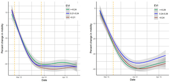
Figure 1. Average daily percent changes in mobility among study areas by EVI level in Maryland (left) and California (right) during the COVID-19 pandemic. Percent change in mobility is the percent change in the number of users traveling in the daytime (8 a.m.–4 p.m.) in a given day compared to the same time and the same day of the week in the reference period (26 February–10 March). Solid line: LOESS smoothing line; grey area: 95% confidence interval of LOESS line; yellow dotted lines for Maryland: declaration of state of emergency and the following stay-at-home order; yellow dotted line for California: stay-at-home order.
Figure 2 shows the descriptive statistics (Q1, Q3, median, and average) of daily percent changes in mobility and EVI values at the MCD level (or CCD level) of the study regions. The scatter plots showed that the regions with high EVI values may have lower reduction in their mobility trend during the study period in Maryland and California. However, the correlation coefficients for the EVI in Maryland were 0.11, −0.01, 0.08, and 0.05 for the Q3, Q1, mean, and median of mobility changes, respectively, indicating no significant correlations. Similarly, for California, no significant correlations were observed for EVI and statistics of mobility changes (0.07, 0.12, 0.08, and 0.08 for the Q3, Q1, mean, and median of mobility changes, respectively).
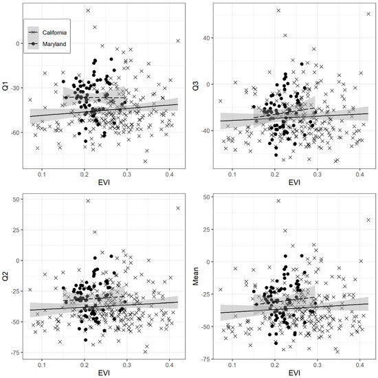
Figure 2. Scatter plots of statistics of percent changes in mobility and EVI in the study areas in Maryland (n = 76) and California (n = 241). The grey area is 95% confidence intervals for linear regression lines.
Figure 3 presents the locations of parks and forest and the geographical patterns of mobility changes (Q3) and EVI. On average, the sizes of parks and forests as well as the size of county subdivisions were larger for California than Maryland. The movement of users was mostly observed in the central areas of Maryland including MCDs adjacent to Baltimore, Maryland. The geographical pattern of EVI showed a relatively particular pattern with higher EVI values for central western parts in Maryland and western parks of California, while the geographical patterns of mobility changes appeared to be random in study regions in both states.
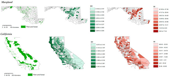
Figure 3. Location of parks and forest and the spatial patterns of EVI and the statistics (Q1, mean, Q3) of percent changes in the number of users moving into each subdivision in Maryland (top) and California (bottom) during the study period (11 March–26 April 2020). Blank area: County subdivisions (MCDs, CCDs) where users’ movement data were unavailable.
Figure 4 presents the mobility change and EVI for MCD (CCD) groups with and without parks. MCDs with parks in Maryland showed slightly lower reduction in mobility compared to MCDs without parks. In California, reduction in mobility was relatively lower in CCDs with parks compared to CCDs without parks. EVI was lower in MCDs and CCDs with parks in Maryland and California.
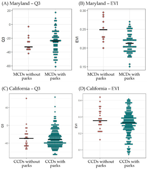
Figure 4. Statistics of percent changes in mobility (Q3) and EVI for MCD (CCD) groups with and without parks in Maryland and California. Solid lines are median.
Regression coefficients of EVI from the linear regression analysis are presented in Table 2. Although MCDs (CCDs) with high EVI values tended to have lower reduction in their mobility (Figure 2), EVI at the MCD (CCD) level in Maryland and California were not significantly associated with mobility changes (Q3) during the study period in any model.
Table 2. Regression coefficients of EVI for the relationship with mobility changes (Q3) in the study county subdivisions (MCD, CCD) in Maryland and California.
| Region | Model 1 | Model 2 | ||||
|---|---|---|---|---|---|---|
| Beta | (95% CI) | p-Value | Beta | (95% CI) | p-Value | |
| Maryland (n = 75) | −1.06 | (−2.49, 0.38) | 0.154 | −1.31 | (−2.63, 0.02) | 0.067 |
| California (n = 241) | 0.02 | (−9.02, 9.74) | 0.933 | 0.13 | (−0.23 0.50) | 0.473 |
Note: EVI = Enhanced Vegetation Index. Model 1 was adjusted for presence of parks (all types), log population density, and number of food retail establishments and hospitals; Model 2 was adjusted for presence of parks (all types), percent impervious area, and number of food retail establishments and hospitals.
Results of the linear regression analysis for presence of parks are shown in Table 3. Presence of state parks in MCD boundary in Maryland was significantly associated with lower reduction in mobility (7.62, 95% CI: 0.28, 14.97) in Model 1, whereas Model 2 and Model 3 did not show significantly lower reduction in mobility. When percent impervious area was included as adjustment instead of population density, having state parks or EVI did not show significant effects on mobility changes. In the third model incorporating the variable of presence of state parks, number of food retail establishments and hospitals, and population density, presence of state parks showed significant effects on mobility changes at a 0.10 significance level. All types of parks and local-scale parks showed no significant relationship with mobility changes in Maryland during the study period. On the other hand, presence of local-scale parks in CCDs in California showed significantly lower reduction in mobility in Model 1 (7.03, 95% CI: 0.12, 13.94) and Model 3 (7.02, 95% CI: 0.13, 13.92). Mobility reduction tended to be lower in CCDs with any type of parks or state or national parks but the results were not significant in California.
Table 3. Results of linear regression analysis on the mobility changes (Q3 and presence of parks in the study county subdivisions (MCD, CCD) in Maryland and California.
| Model 1 | Model 2 | Model 3 | |||||||
|---|---|---|---|---|---|---|---|---|---|
| Variable | Beta | (95% CI) | p-Value | Beta | (95% CI) | p-Value | Beta | (95% CI) | p-Value |
| Maryland (n = 75) | |||||||||
| Presence of parks by type (ref = having no park) | |||||||||
| Total | 7.31 | (−4.97, 1.96) | 0.248 | 1.57 | (−9.96, 13.10) | 0.790 | 7.00 | (−4.61, 18.60) | 0.242 |
| State and National | 7.62 | (0.27, 14.97) | 0.045 | 5.56 | (−1.87, 13.00) | 0.145 | 6.04 | (−1.05, 13.13) | 0.100 |
| Local | 5.79 | (−5.21, 16.80) | 0.306 | 0.057 | (−9.52, 10.65) | 0.913 | 5.71 | (−4.87, 16.29) | 0.294 |
| California (n = 241) | |||||||||
| Presence of parks by type (ref = having no park) | |||||||||
| Total | 0.36 | (−9.02, 9.75) | 0.939 | −0.04 | (−9.71, 8.87) | 0.930 | 0.33 | (−9.00, 9.66) | 0.945 |
| State and National | 0.22 | (−6.20, 6.65) | 0.946 | 0.38 | (−5.91, 6.68) | 0.906 | 0.20 | (−6.19, 6.58) | 0.952 |
| Local | 7.03 | (0.12, 13.94) | 0.048 | 5.17 | (−1.01, 11.36) | 0.102 | 7.02 | (0.13, 13.92) | 0.047 |
Note: Model 1 was adjusted for number of food retail establishments and hospitals, population density, and EVI; Model 2 was adjusted for number of food retail establishments and hospitals, percent impervious area, and EVI; Model 3 was adjusted for number of food retail establishments and hospitals and log population density.
This entry is adapted from the peer-reviewed paper 10.3390/su12229401