Your browser does not fully support modern features. Please upgrade for a smoother experience.
Please note this is an old version of this entry, which may differ significantly from the current revision.
In order to safeguard image copyrights, zero-watermarking technology extracts robust features and generates watermarks without altering the original image. Traditional zero-watermarking methods rely on handcrafted feature descriptors to enhance their performance.
- zero-watermarking
- deep learning
- robustness
- discriminability
1. Introduction
In contrast to cryptography, which primarily focuses on ensuring message confidentiality, digital watermarking places greater emphasis on copyright protection and tracing [1,2]. Classical watermarking involves the covert embedding of a watermark (a sequence of data) within media files, allowing for the extraction of this watermark even after data distribution or manipulation, enabling the identification of data sources or copyright ownership [3]. However, this embedding process necessarily involves modifications to the host data, which can result in some degree of degradation to data quality and integrity. In response to the demand for high fidelity and zero tolerance for data loss, classical watermarking has been supplanted by zero-watermarking. Zero-watermarking focuses on extracting robust features and their fusion with copyright information [4,5]. Notably, a key characteristic of zero-watermarking lies in the generation or construction of the zero-watermark itself, as opposed to its embedding.
Commonly, zero-watermarking algorithms are traditionally reliant on handcrafted features and typically involve a three-stage process. The first stage entails computing robust features, followed by converting these features into a numerical sequence in the second stage. The third stage involves fusing the numerical sequence with copyright identifiers, resulting in the generation of a zero-watermark without any modifications to the original data. Notably, the specific steps and features in these three stages are intricately designed by experts or scholars, thereby rendering the performance of the algorithm contingent upon expert knowledge. Moreover, once a zero-watermarking algorithm is established, continuous optimization becomes challenging, representing a limitation inherent in handcrafted approaches.
Introducing deep learning technology is a natural progression to overcome the reliance on expert knowledge and achieve greater optimization in zero-watermarking algorithms. Deep learning has recently ushered in significant transformations in computer vision and various other research domains [6,7,8,9]. Numerous tasks, including image matching, scene classification, and semantic segmentation, have exhibited remarkable improvements when contrasted with classical methods [10,11,12,13,14]. The defining feature of deep learning is its capacity to replace handcrafted methods reliant on expert knowledge with Artificial Neural Networks (ANNs). Through training ANNs with ample samples, these networks can effectively capture the intrinsic relationships among the samples and model the associations between inputs and outputs. Inspired by this paradigm shift, the zero-watermarking method can also transition towards an end-to-end mode with the support of ANNs, eliminating the need for handcrafted features.
2. Zero-Watermarking
The concept of zero-watermarking in image processing was originally introduced by Wen et al. [15]. This technology has garnered significant attention and research interest due to its unique characteristic of preserving the integrity of media data without any modifications. Taking images as an example, the zero-watermarking process can be broadly divided into three stages. The first stage involves the computation of robust features. In this phase, various handcrafted features such as Discrete Cosine Transform (DCT) [16,17], Discrete Wavelet Transform (DWT) [18], Lifting Wavelet Transform [19], Harmonic Transform [5], and Fast Quaternion Generic Polar Complex Exponential Transform (FQGPCET) [20] are calculated and utilized to represent the stable features of the host image. The second stage focuses on the numerical conversion of these features into a numerical sequence. Mathematical transformations such as Principal Component Analysis (PCA) and Singular Value Decomposition (SVD) are employed to filter out minor components and extract major features [16,21]. The resulting feature sequence from this stage serves as a condensed identifier of the original image. However, this sequence alone cannot serve as the final watermark since it lacks any copyright-related information. Hence, the third stage involves the fusion of the feature sequence with copyright identifiers. Copyright identifiers can encompass the owner’s signature image, organization logos, text, fingerprints, or any digitized media. To ensure the zero-watermark cannot be forged or unlawfully generated, cryptographic methods such as Advanced Encryption Standard (AES) or Arnold Transformation [22] are often utilized to encrypt the copyright identifier and feature sequence. The final combination can be as straightforward as XOR operations [16]. Consequently, the zero-watermark is generated and can be registered with the Intellectual Property Rights (IPR) agency. Additionally, copyright verification is a straightforward process involving the regeneration of the feature sequence and its comparison with the registered zero-watermark. The process of zero-watermarking technology is illustrated in Figure 1.
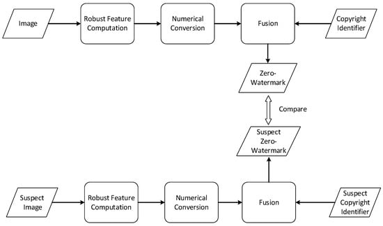
Figure 1. The process of zero-watermark generation and verification.
Presently, several research efforts focus on deep-learning-based watermarking methods, encompassing both classical watermarking of embedding style and zero-watermarking of generative style. In the domain of embedding-style watermarking, a method inspired by the architecture of Autoencoder has been proposed. In this approach, Autoencoders encode the watermark and embed it using convolutional networks. For watermark extraction, Autoencoders are also employed to extract and decode the watermark [23]. Other Autoencoder-based methods aim to enhance robustness or improve efficiency [24,25]. Despite their superior performance in robustness and elimination of reliance on prior knowledge, embedding-style watermarking significantly differs from zero-watermarking methods, as the latter maintains the original data unchanged. Additionally, it is noteworthy that zero-watermarking places greater emphasis on discriminability, a focus less pronounced in embedding-style watermarking.
In the realm of deep-learning-based zero-watermarking methods, a hybrid scheme that combines traditional Discrete Wavelet Transform (DWT) and the deep neural network ResNet-101 has been proposed. This approach involves applying DWT to the host image and subsequently sending the wavelet coefficients to ResNet-101 [26]. While exhibiting strong robustness against translation and clipping, this scheme falls short of being an end-to-end solution. Regarding end-to-end zero-watermarking, some studies employ Convolutional Neural Networks (CNN), VGG-19 (developed by the Oxford Visual Geometry Group), or DenseNet to generate robust watermark sequences [27,28,29]. Another line of research predominantly revolves around the concept of style transfer [30]. In the watermark generation phase, it utilizes VGG to merge the content of the copyright logo with the style of the host image. In the verification stage, another CNN is employed to eliminate the style component and extract the copyright content. Although these approaches have demonstrated promising levels of robustness compared to handcrafted methods, we believe they fall short in adequately considering multi-level features within the image. This limitation arises because when using CNN or VGG to upsample the image, the higher-level features have a less effective receptive field than the theoretical receptive field [31]. Furthermore, one drawback of these zero-watermark networks is the insufficient emphasis on discriminability. This means the generated zero-watermarks for different images should be distinct enough to prevent copyright ambiguity.
3. ConvNeXt
Convolutional Neural Networks (CNN) have been employed as the feature extraction component in existing watermarking methods. However, it is noteworthy that the performance of CNN has become outdated in various tasks. Hence, Liu et al. introduced ConvNeXt, a nomenclature devised to distinguish it from traditional Convolutional Networks (ConvNets) while signifying the next evolution in ConvNets [32]. Rather than presenting an entirely new architectural paradigm, ConvNeXt draws inspiration from the ideas and optimizations put forth in the Swin Transformer [33] and applies similar strategies to enhance a standard ResNet [8]. These optimization strategies can be summarized as follows:
(1) Modification of stage compute ratio: ConvNeXt adjusts the number of blocks within each stage from (3, 4, 6, 3) to (3, 3, 9, 3).
(2) Replacement of the stem cell: The introduction of a patchify layer achieved through non-overlapping 4 × 4 convolutions.
(3) Utilization of grouped and depthwise convolutions.
(4) Inverted Bottleneck design: This approach involves having the hidden layer dimension significantly larger than that of the input.
(5) Incorporation of large convolutional kernels (7 × 7) and depthwise convolution layers within each block.
(6) Micro-level optimizations: These include the replacement of ReLU with GELU, fewer activation functions, reduced use of normalization layers, the substitution of Batch Normalization with Layer Normalization, and the implementation of separate downsampling layers.
Remarkably, the amalgamation of these strategies results in ConvNeXt achieving a state-of-the-art level of performance in image classification, all without requiring substantial changes to the network’s underlying structure. Furthermore, a key feature of this paper lies in its detailed presentation of how each optimization incrementally enhances performance, effectively encapsulated in Figure 2.
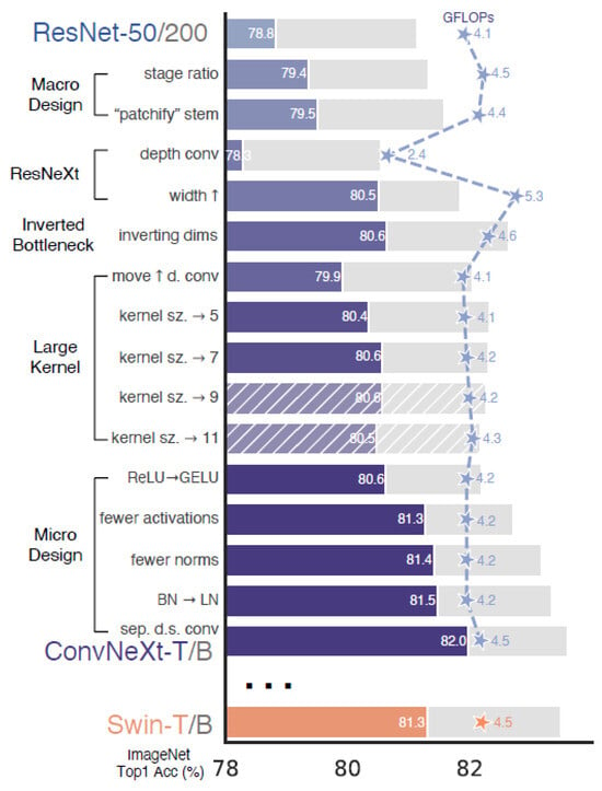
Figure 2. Incremental improvement through optimization steps in ConvNeXt [32]. The foreground bars represent results from ResNet-50/Swin-T, while the gray bars represent results from ResNet-200/Swin-B.
From Figure 2, it is evident that employing the strategy of stage ratio modification and patchify stem leads to an improvement in accuracy, increasing from 78.8% to 79.5%. Further enhancements are observed with the introduction of depth convolution and larger width, resulting in an accuracy improvement of 80.5%. The utilization of an inverted bottleneck and larger kernel size contributes to a higher accuracy of 80.6%. Finally, with micro-optimizations, the accuracy of ConvNeXt reaches 82.0%, surpassing that of Swin.
4. LK-PAN
While ConvNeXt offers a straight-line structure that effectively captures local features, it may fall short in dedicating sufficient attention to the global context. To address this limitation and enhance the capabilities of ConvNeXt, a path aggregation mechanism, LK-PAN, is introduced. LK-PAN originates from the Path Aggregation Network (PANet), which was initially introduced in the context of instance segmentation to bolster the hierarchy of feature extraction networks. The primary structure of PANet is depicted in Figure 3.
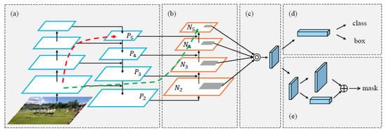
Figure 3. The primary structure of PANet [34]. (a) The backbone part of PANet; (b) Bottom-up path augmentation; (c) Adaptive feature pooling; (d) Box branch; (e) Fully-connected fusion.
In Figure 3, we observe that part (a) represents the classical network structure of the Feature Pyramid Network (FPN), which is named for its pyramid-like arrangement [35]. However, it’s important to note that the influence of low-level features on high-level features is limited due to the long paths, as indicated by the red dashed lines in Figure 3. These paths can comprise over 100 layers. While the theoretical receptive field of P5 may be quite large, it does not manifest as such in practice due to the numerous convolution, pooling, and activation operations. Therefore, PANet introduced a bottom-up path augmentation, as depicted in Figure 3b. This approach aggregates the top-most features from both the low-level features and features at the same level. Consequently, this mechanism substantially shortens the connection between low-level features and the top-most features to around 10 layers. Thus, it effectively enhances feature expression for local areas and minor details. PANet’s contributions also encompass adaptive feature pooling (Figure 3c) and fully-connected fusion (Figure 3d). However, these two mechanisms are more closely related to the task of instance segmentation and will not be elaborated upon here.
Building upon the foundation of PANet, the Large Kernel-PANet, abbreviated as LK-PAN [36], introduces some improvements. The primary feature of LK-PAN is the enlargement of the convolution kernel size. In contrast to PANet, LK-PAN utilizes 9 × 9 convolution kernels instead of the original 3 × 3 size. This augmentation is aimed at expanding the receptive field of the feature map, thereby enhancing the ability to discern minor features with greater precision. Another key change in LK-PAN is the adoption of a concatenation operation, replacing Figure 3c, for fusing features from different levels.
This entry is adapted from the peer-reviewed paper 10.3390/app14010435
This entry is offline, you can click here to edit this entry!