Your browser does not fully support modern features. Please upgrade for a smoother experience.
Please note this is an old version of this entry, which may differ significantly from the current revision.
The fundamental principles and structures of deep learning (DL) are examined herein. The specific roles and functions of the diverse layers that make up deep networks are discussed, and the importance of evaluation metrics, which serve as crucial tools for gauging the effectiveness of these models, are emphasized. Commonly used architectures in medical image segmentation are also introduced.
- deep learning
- segmentation
- evaluation metrics
- medical image segmentation
1. Deep Neural Network Architectures
1.1. Convolutional Neural Networks (CNNs)
Convolutional Neural Networks (CNNs) have established themselves as some of the most impactful and commonly used architectures within the DL networks, particularly for tasks related to computer vision. Waibel et al. [53] further developed CNNs by introducing shared weights across temporal receptive fields and using backpropagation training for phoneme recognition. LeCun et al. [54] also contributed to the field by designing a CNN architecture specifically for the task of document recognition.
Convolution is a critical mathematical operation within the structure of CNNs. It operates linearly, taking input data and multiplying it by specified weights. This operation is executed with the assistance of a filter or mask, which is essentially a two-dimensional weight array and is generally smaller than the input data. The procedure entails conducting an element-wise multiplication, or dot product, between the filter and an equivalent-sized patch of the input. This results in a single output value. This process is systematically replicated across the whole input image, creating a two-dimensional output array known as a feature map. A notable aspect of this operation is the consistent application of the same filter across the entire image, allowing the algorithm to identify a particular feature regardless of its position in the image. This key feature is referred to as translation invariance.
A key strength of CNNs is their capability to self-learn filters, eliminating the necessity for manual filter creation. By leveraging the power of backpropagation, an essential training technique, the network adjusts the weights of the filters based on the error it calculates during the training phase. This advantage provides a more dynamic and adaptive approach to identifying relevant features within the data.
The learning process occurs across various layers, each responsible for identifying distinct types of features within the data. The layers closer to the input are typically tasked with learning low-level features such as lines and edges, serving as the building blocks for more complex pattern recognition. As we move deeper into the network, the layers progressively learn to recognize more complex, higher-order features like shapes and object parts. This hierarchical learning structure allows the model to gradually construct a more intricate understanding of the input data, from simple, foundational elements to complex, composite features. A representation of the CNN general workflow is provided in Figure 2.
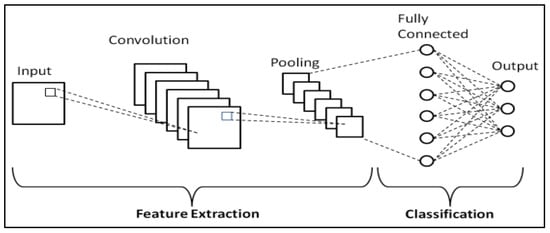
Figure 2. Schematic representation of CNNs [55].
1.2. Recurrent Neural Networks (RNNs)
Recurrent Neural Networks (RNNs) [56] represent another class of DL architectures that have shown significant promise in tasks involving sequential data. Each neuron in a layer of an RNN receives input not only from the previous layer but also from its previous time step, enabling the model to exhibit temporal dynamic behavior and recognize patterns across time. This makes them particularly adept for tasks such as natural language processing, speech recognition, machine translation, music generation, and sentiment classification, where the order of the input data carries significant information. Key advantages of RNNs include their ability to process inputs of any length and maintain compact model size, regardless of the larger inputs. However, RNNs do face challenges, including higher computational costs, difficulty in accessing distant past information, and issues related to the vanishing or exploding gradient problem.
Vanishing and exploding gradients are common issues encountered during the training of neural networks, particularly those with deep architectures like RNNs. Both problems can make it difficult for an RNN to learn and maintain long-term dependencies in the data. To address this, Long Short-Term Memory (LSTM) [57] networks and Gated Recurrent Unit (GRU) [58] were introduced. A depiction of the general workflow of RNNs can be seen in Figure 3.
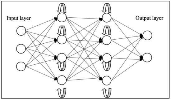
Figure 3. Schematic representation of RNNs [59].
1.3. Encoder–Decoder Network Models
Encoder–Decoder models are a class of DL models that have shown significant results in a variety of tasks. These models consist of two main components: an encoder model that is responsible for compressing data into a compact latent representation, and a decoder model that reconstructs the original data from this latent representation. The overall goal of these models is to learn a representation of the data that can capture its structure. A notable application of encoder–decoder models can be found in medical imaging. The study titled “Low-Dose CT With a Residual Encoder-Decoder Convolutional Neural Network” by Hu Chen and colleagues (2017) [60] showcases a model that integrates an autoencoder, deconvolution network, and shortcut connections to form a residual encoder–decoder convolutional neural network (RED-CNN), specifically designed for low-dose CT imaging. The model was trained on patch-based data and demonstrated competitive performance in terms of noise suppression, structural preservation, and lesion detection.
1.4. Generative Adversarial Networks (GANs)
Generative Adversarial Networks (GANs) are a groundbreaking and potent methodology used in unsupervised and semi-supervised learning [61]. GANs, a relatively recent innovation, draw inspiration from noise-contrastive estimation and harness implicit modeling of high-dimensional data distributions. The structure of GANs is bifurcated into two neural networks: a generative network, tasked with learning the patterns within a database to synthesize plausible new data, and a discriminative network, which categorizes samples as either original or generated data. These two networks participate in a competitive interplay, where the loss of one network equates to the gain of the other. The fundamental principle of GANs is to motivate the generator to produce a data distribution that closely mirrors that of real data, with the generative networks being indirectly trained with a dynamically updated discriminative network.
Since their introduction, GANs have been extensively applied across a wide range of tasks in computer vision, including image segmentation. Various GAN architectures have been developed and deployed, such as fully connected GANs [62], Convolutional GANs [63], Conditional GANs [64], Wasserstein-GAN [65], GANs with inference models, and Adversarial autoencoders. The adaptability and effectiveness of GANs have led to their incorporation in numerous studies and projects, showcasing their potential to enhance accuracy and enable semi-weakly supervised semantic segmentation. As the field continues to progress, GANs are anticipated to assume an increasingly pivotal role in the advancement of deep learning and computer vision. A visual representation of the general workflow of GANs is illustrated in Figure 4.
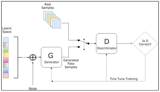
Figure 4. Schematic representation of GANs [66].
2. Deep Neural Network Layers
2.1. Activation Layer
In deep learning models, the activation layer is essential as it determines the necessary information for accurate predictions. Typically found after the convolutional layers in CNNs, these layers function on feature maps. The activation function within these layers decides if a neuron’s input should be activated based on the input’s significance for the model’s prediction accuracy. These functions must be efficient due to the fact that they will be applied across millions of neurons. Moreover, in CNNs, backpropagation requires these functions to be non-linear, demanding additional computational efficiency. Over the years, several activation functions such as sigmoid [67], softmax [68], Rectified Linear Units (ReLU) [69], Leaky ReLU [70], and the recently introduced Swish [71] have been developed.
The sigmoid function,
which ranges from 0 to 1, is ideal for models predicting probabilities. The SoftMax function
is a more general sigmoid function commonly used for multi-class classification. However, these functions can be computationally intensive and may face the issue of vanishing gradients.
ReLU is a widely used activation function because of its simplicity and ability to handle the vanishing gradient problem. However, it can experience the “dying ReLU” problem as it outputs zero for all negative inputs, inhibiting backpropagation.
Leaky ReLU, an improved version of ReLU, addresses this problem but may introduce some inconsistencies for negative input predictions. Both Leaky ReLU and ReLU can still encounter the exploding gradient problem with larger input values.
Parametric ReLUs (PReLUs)
extend this concept by transforming the leakage coefficient into a parameter that is learned concurrently with the other parameters of the neural network. Here, α is a learnable parameter. This innovative approach allows the network to self-adjust the coefficient based on the specific requirements of the data, thereby enhancing the adaptability and performance of the model.
Lastly, the Swish function,
a further improvement of ReLU developed by Google researchers, maintains computational efficiency and can sometimes outperform ReLU.
2.2. Pooling and Batch Normalization
Pooling layers are a crucial component of CNNs. Pooling layers are generally placed between consecutive convolutional layers within a CNN architecture. Their main role is to diminish the spatial dimensions of the representation, which in turn reduces the number of parameters and computational load in the network. This controls overfitting and makes the network invariant to small translations. Multiple types of pooling operations exist, with Max pooling and average pooling being the most commonly utilized.
Max pooling is the most common type of pooling, and it involves defining a spatial neighborhood (for example, a 2 × 2 window) and taking the largest element from the rectified feature map within that window. Instead of taking the average element value, we take the maximum element. This highlights the most present feature in the local region of the feature map. Max pooling has been favored in practice due to its performance in experiments and its ability to preserve the presence of the feature, no matter how small. Average pooling is a process that computes the average value for each patch on the feature map. This means that each max pooling operation (over a 2 × 2 window) is replaced with an unweighted average over the same window. This was often used traditionally but has recently been largely replaced with max pooling, which performs better in practice.
Pooling layers provide a form of translation invariant representation in the feature map, which can be beneficial in image classification tasks where objects may appear in different locations of the input image1. Pooling layers contribute to making the representation approximately invariant to minor translations of the input. This translation invariance is particularly beneficial when the presence of a feature is more significant than its precise location. Batch normalization [72] is a strategy used for efficiently training deep neural networks. It involves standardizing the inputs to a specific layer across each mini-batch, thereby stabilizing the learning process and markedly decreasing the number of epochs required to train deep networks. This technique was introduced to tackle the issue of internal covariate shift, a phenomenon where the distribution of inputs for each layer shifts during the training process due to changes in the parameters of preceding layers. This can slow down the training process and make it difficult to train models with saturating nonlinearities. It has been shown to have a dramatic effect on the optimization performance of neural networks. Moreover, batch normalization can also act as a form of regularization, effectively reducing the generalization error, similar to how activation regularization functions.
2.3. Optimizers
Optimizers play a crucial role in deep learning, as they are responsible for updating the weight parameters and minimizing the loss function. They are the driving force behind the training of deep learning models, and their efficiency can significantly impact the performance of these models. In the context of deep learning, several optimizers have been developed to improve the performance of models.
Stochastic Gradient Descent (SGD) [73] is one of the most basic optimization algorithms in deep learning. It uses a fixed learning rate for all parameters throughout the entire training process, and it is known for its fast convergence ability.
The Adaptive Gradient Algorithm (Adagrad) [74] is an optimizer that uses different learning rates for each parameter in the model. It adapts the learning rate according to the frequency of each parameter’s update, which can be particularly beneficial for dealing with sparse data and large-scale problems.
Root Mean Square Propagation (RMSProp) [75] is an optimization algorithm designed to address the diminishing learning rates in Adagrad. RMSProp uses an exponentially decaying average to discard history from the extreme past, allowing it to converge rapidly after finding a convex bowl.
Adadelta [76] builds upon Adagrad’s framework, aiming to mitigate its steeply declining learning rate. Unlike Adagrad, which accumulates all historical squared gradients, Adadelta limits the scope of these gradients to a constant window, denoted as ‘w’. This is achieved by setting the state as a progressively diminishing average of past squared gradients. Adam (Adaptive Moment Estimation) [77] is another popular optimizer that computes adaptive learning rates for different parameters. It stores an exponentially decaying average of past gradients similar to momentum and RMSProp. This characteristic renders it particularly effective for problems with large datasets or a high number of parameters.
DL optimizers are essential for effectively training models and achieving high performance. The choice of optimizer can significantly impact the model’s ability to learn from the data and generalize well to unseen data.
2.4. Fully Connected Layers
Fully connected layers, also known as dense layers, play a crucial role in the architecture of neural networks. These layers are characterized by their interconnectivity, where each neuron in a layer is connected to all neurons in the previous layer. This dense interconnection allows for the integration of learned features from prior layers, thus enabling the network to learn more complex representations. Fully connected layers are typically used toward the end of a neural network, following several convolutional or recurrent layers that are responsible for feature extraction. The role of the fully connected layers is to take these extracted features and combine them in various ways to solve the problem the network is designed to address, such as classification or segmentation [78].
2.5. Dropout Layer
Dropout layers [79] are a powerful and intuitive regularization technique. Dropout operates on the principle of randomly omitting units and their connections within the neural network during the training phase. By doing so, it hinders excessive co-adaptation among units, resulting in a network with enhanced generalization capabilities. During training, dropout effectively trains a large ensemble of thinned networks with shared weights, where each thinned network gets trained very rarely, if at all. This effectiveness stems from the fact that with each instance of training, a newly ‘thinned’ version of the network is generated and subjected to training. The thinned networks are derived from the original network by removing non-output units independently with a certain probability during the training phase. Dropout has demonstrated a notable ability to curb overfitting, yielding substantial enhancements compared with other regularization techniques.
3. Evaluation Metrics
Assessment metrics are vital for evaluating the effectiveness of semantic segmentation models in deep learning. These metrics provide quantitative measures that reflect the accuracy and effectiveness of the model in segmenting images. They are essential in comparing different models, tuning model parameters, and improving model performance. In the medical imaging field, these metrics are particularly important due to the high precision required in tasks such as tumor detection and organ delineation. The choice of evaluation metric can significantly impact the perceived performance of a model and guide the development of more effective models. The following sections will delve into some of the most popular and widely used evaluation metrics for semantic segmentation.
3.1. Precision
Precision [80], often referred to as the positive predictive value, is a critical evaluation metric in semantic segmentation tasks, particularly in the context of medical imaging. Precision is defined as the ratio of true positive predictions (i.e., the number of pixels correctly identified as belonging to a particular class) to the total number of positive predictions made by the model, which includes both true positives and false positives (i.e., the number of pixels incorrectly identified as belonging to that class). Mathematically, it can be expressed as:
Precision provides an estimate of how many of the pixels that the model classifies as belonging to a particular class are actually of that class. A model with high precision demonstrates a low rate of false positives, which is especially valuable in scenarios where the consequences of false positives are significant. However, it is important to note that precision does not take into account false negatives (i.e., pixels of a particular class that the model fails to identify), and thus should be considered alongside other metrics such as recall (or sensitivity) for a more comprehensive evaluation of model performance.
3.2. Recall
Recall [80], also known as sensitivity or true positive rate, is another vital evaluation metric in the domain of semantic segmentation, particularly in medical imaging applications. Recall is defined as the ratio of true positive predictions (i.e., the number of pixels correctly identified as belonging to a specific class) to the actual number of pixels that truly belong to that class, which includes both true positives and false negatives (i.e., the number of pixels that are incorrectly identified as not belonging to that class). Mathematically, it can be expressed as:
Recall provides an estimate of the model’s ability to correctly identify all pixels of a particular class. When a model exhibits high recall, it means it has a low rate of false negatives, which is particularly advantageous in situations where avoiding false negatives is crucial. However, it is important to note that recall does not take into account false positives (i.e., pixels that the model incorrectly identifies as belonging to a particular class) and thus should be used in conjunction with other metrics such as precision for a more comprehensive evaluation of model performance.
3.3. F-Measure
The F-measure [81], also known as the F1 score, is a widely used evaluation metric in semantic segmentation, particularly in the field of medical imaging. The F-measure is the harmonic mean of precision and recall, two critical metrics that respectively measure the model’s ability to avoid false positives and false negatives. By combining precision and recall, the F_measure provides a single metric that balances the trade-off between these two aspects. Mathematically, it can be expressed as:
The F-measure offers a comprehensive measure of the model’s performance. A high F-measure indicates that both the precision (i.e., the model’s ability to correctly identify pixels of a particular class without incorrectly classifying other pixels as belonging to that class) and the recall (i.e., the model’s ability to correctly identify all pixels of a particular class) are high. This makes the F-measure particularly useful when it is equally important to minimize both false positives and false negatives.
3.4. Dice Coefficient
The Dice coefficient [82], also known as the Sørensen–Dice index or Dice similarity coefficient (DSC), is a prominent evaluation metric used in semantic segmentation, particularly in the field of medical imaging. The Dice coefficient measures the overlap between two samples and is particularly useful for comparing the pixel-wise agreement between a predicted segmentation and its corresponding ground truth.
Mathematically, the DSC is calculated by doubling the area of overlap between the predicted and actual ground truth segments and then dividing by the sum of the total pixel counts in both the predicted and ground truth segments.
The Dice coefficient provides an estimate of the model’s ability to correctly identify the boundaries of a particular class. A high Dice coefficient indicates a high degree of overlap between the predicted and actual segments, suggesting that the model accurately identifies the boundaries of the class.
3.5. Intersection over Union
Intersection over Union (IoU) [82], also known as the Jaccard index, is a commonly used evaluation metric in semantic segmentation, particularly in the field of medical imaging. IoU measures the overlap between the predicted segmentation and the ground truth by dividing the area of overlap by the area of union.
Mathematically, IoU is determined by dividing the area of overlap between the predicted and ground truth segments by the area of their union. It can be expressed as:
IoU provides an estimate of the model’s ability to correctly identify both the location and extent of a particular class. A high IoU indicates a high degree of overlap between the predicted and actual segments, suggesting that the model accurately identifies the location and extent of the class.
3.6. Area Under the Curve
The Area Under the Curve (AUC) [81], specifically, the Receiver Operating Characteristic (ROC) curve, is a widely used evaluation metric in semantic segmentation, particularly in the field of medical imaging. The ROC curve represents a graph that demonstrates the diagnostic capability of a binary classification system across varying discrimination thresholds. The Area Under the Curve (AUC) offers a quantification of the model’s proficiency in differentiating between positive and negative classes.
Mathematically, the AUC is the integral of the ROC curve, and it quantifies the overall performance of a model across all possible classification thresholds. An AUC of 1 indicates a perfect classifier, while an AUC of 0.5 suggests a random classifier.
AUC provides an aggregate measure of the model’s performance across different levels of sensitivity and specificity. A high AUC indicates that the model has a high true positive rate for a given false positive rate across various threshold settings.
4. Medical Image Segmentation Architectures
With the advent of deep learning, a variety of architectures have been proposed and developed specifically for medical image segmentation, offering significant improvements in accuracy and efficiency over traditional methods.
4.1. Fully Convolutional Networks
Fully Convolutional Networks (FCNs) [83] have emerged as powerful and efficient approaches to semantic segmentation. FCNs are a class of models within the broader family of convolutional networks, which have been instrumental in driving advances in image recognition tasks. The primary innovation of Fully Convolutional Networks (FCNs) lies in their capacity to process inputs of any size and generate outputs with corresponding dimensions while maintaining efficient inference and learning. A distinctive characteristic of Fully Convolutional Networks (FCNs) is their capability to integrate deep, broad semantic details with shallow, detailed appearance information. This is achieved with a novel architecture that includes in-network upsampling layers, which enable pixel-wise prediction and learning in networks with subsampled pooling. This combination of deep and shallow information allows FCNs to make local predictions that respect the global structure of the image.
One of the primary advantages of FCNs for semantic segmentation is their ability to provide an end-to-end solution, even when dealing with images of varying sizes. This feature, combined with their other strengths, makes FCNs highly effective tools in the field of semantic segmentation. The limitations of FCNs encompass their substantial computational demands and the challenges they face when adapting to three-dimensional imagery. The architecture of an FCN is depicted in Figure 5.
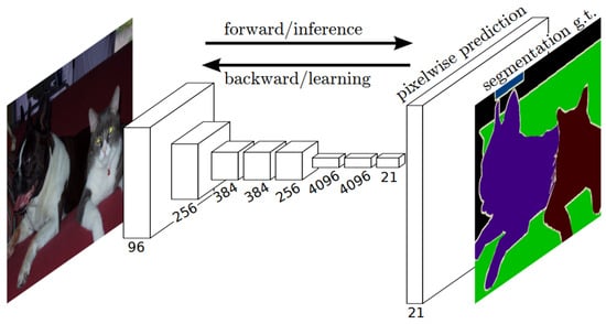
Figure 5. Schematic representation of an FCN [83].
4.2. U-Net
U-Net [84] is another influential architecture that has made significant strides in the field of semantic segmentation, particularly in biomedical image processing. The architecture is designed as an encoder–decoder network, with the encoder extracting features from the input image and the decoder using these features to generate a segmentation map. The U-Net architecture is characterized by its symmetric structure. The encoding path progressively captures the context in the image, while the decoding path helps in precise localization using transposed convolutions. Thus, U-Net combines the advantages of both local features and the global context, which is crucial for accurate semantic segmentation. A distinctive feature of U-Net is the introduction of skip connections between the encoder and decoder. These skip connections allow the network to use information from the earlier layers in the later layers, which helps in recovering the full spatial resolution of the output. This is particularly useful in tasks like medical image segmentation, where every pixel can be important.
U-Net offers several advantages for semantic segmentation. It provides an efficient way to deal with the limited amount of annotated images in the medical field, as it can be trained with relatively few images and still deliver high segmentation accuracy. Furthermore, the use of skip connections allows U-Net to capture both high-level and low-level features, leading to more precise segmentation. The structure of the U-Net architecture is demonstrated in Figure 6.
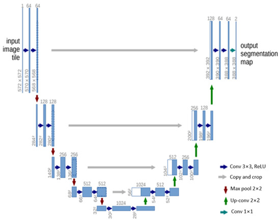
Figure 6. Schematic representation of the U-Net [84].
4.3. V-Net
V-Net [85] is a powerful architecture designed specifically for volumetric medical image segmentation. This refers to a 3D adaptation of the U-Net architecture, specifically crafted to work directly with 3D images. This feature is especially beneficial in medical imaging contexts, where data frequently comprise 3D volumes like MRI or CT scans. The architecture of V-Net is characterized by its symmetric structure. Comparable to the U-Net architecture but with notable distinctions, this network is segmented into various stages, each functioning at different resolutions. Each stage consists of one to three convolutional layers, and a residual function is learned at every stage. Such an architecture enhances the likelihood of convergence compared with networks that do not incorporate residual learning. A distinctive aspect of the V-Net architecture is its use of volumetric kernels in the convolutions executed at each stage. This enables the model to effectively grasp three-dimensional spatial information, essential for precise segmentation in three-dimensional medical imaging. During the compression pathway, the resolution is decreased using convolution with 2 × 2 × 2 voxel-wide kernels, applied with a stride of 2, akin to the pooling layers found in other network architectures. The configuration of the V-Net architecture is depicted in Figure 7.
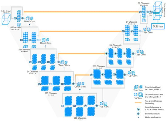
Figure 7. Schematic representation of the V-Net [85].
4.4. U-Net++
U-Net++ [86] is an enhanced version of the U-Net architecture, designed to address some of the limitations of the original U-Net. The U-Net++ architecture introduces several innovative features that enhance its performance in semantic segmentation tasks, particularly in the field of medical imaging.
The architecture is characterized by its dense convolutional blocks and deep supervision design. The dense convolutional blocks are designed to reduce the semantic gap between the feature maps of the encoder and decoder, making the learning task easier for the model. These blocks take into account not only the information from the previous nodes in the same level but also the nodes in the level below it. This dense connectivity allows the model to capture both high-level and low-level features, leading to more precise segmentation. The deep supervision design of U-Net++ allows the model to operate in two modes: the accurate mode and the fast mode. In the accurate mode, the outputs from all branches in level 0 are averaged to produce the final result. In the fast mode, not all branches are selected for outputs. This flexibility allows U-Net++ to adapt to different computational and accuracy requirements.
U-Net++ offers several advantages for semantic segmentation. The use of dense connections and deep supervision allows U-Net++ to capture both high-level and low-level features, leading to more precise segmentation. The structure of the U-Net++ architecture is demonstrated in Figure 8.
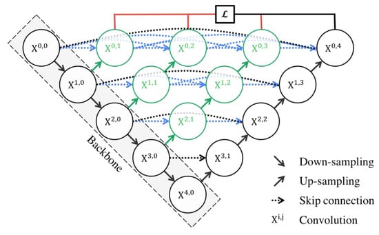
Figure 8. Schematic representation of the U-Net++ [86].
4.5. Attention U-Net
The Attention U-Net [87] presents an innovative approach to image segmentation by incorporating an attention gate (AG) mechanism. This mechanism enables the model to concentrate on specific target structures within an image, thereby enhancing its generalization capability and reducing computational waste on irrelevant activations.
The attention mechanism can be categorized into two types: hard and soft. Hard attention, although effective in highlighting relevant regions, is non-differentiable and necessitates the use of reinforcement learning for training. Conversely, soft attention assigns weights to different regions of the image based on their relevance, allowing for differentiation and training using standard backpropagation. This method ensures that the model focuses more on regions with higher weights during the training process.
The integration of attention into the U-Net architecture addresses the issue of imprecise spatial information during the upsampling phase. U-Net uses skip connections to combine spatial information from both the downsampling and upsampling paths. However, this process often results in the propagation of redundant low-level features. The application of soft attention at these skip connections effectively suppresses activations in irrelevant regions, thereby reducing feature redundancy.
Attention gates utilize additive soft attention, taking two input vectors: x and g. The vector g, derived from the next lower layer of the network, possesses superior feature representation due to its origin deeper within the network. These vectors undergo an element-wise summation, followed by a ReLU activation layer and a 1 × 1 convolution. The resulting vector is then scaled within the range of [0, 1] through a sigmoid layer, producing the attention coefficients. These coefficients, indicative of feature relevance, are then upsampled to the original dimensions of the x vector and multiplied element-wise to the original x vector, effectively scaling the vector based on relevance. The schematic representation of the Attention U-Net architecture can be seen in Figure 9.
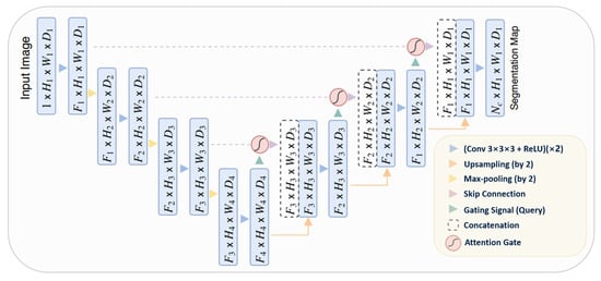
Figure 9. Schematic representation of the Attention U-Net [87].
4.6. ResUNet++
ResUNet++ [88], an enhanced version of the ResUNet architecture, has been developed specifically for medical image segmentation tasks, with a particular focus on pixel-wise polyp segmentation in colonoscopy examinations. The architecture integrates multiple sophisticated elements, such as residual blocks, squeeze and excitation blocks, Atrous Spatial Pyramidal Pooling (ASPP), and attention blocks, enhancing its overall functionality and efficiency. ResUNet++ is based on the Deep Residual U-Net (ResUNet) framework, combining the advantages of deep residual learning with the U-Net structure. Its architecture consists of a stem block, three encoder blocks, an Atrous Spatial Pyramidal Pooling (ASPP) section, and three decoder blocks. In each encoder block of this architecture, there are two consecutive 3 × 3 convolutional blocks followed by identity mapping. A strided convolution layer is then used to reduce the spatial dimensions of the feature maps. Subsequently, the output goes through a squeeze-and-excitation block. The Atrous Spatial Pyramidal Pooling (ASPP) functions as a bridge, offering a wider contextual perspective. The decoding path mirrors the encoding path, utilizing residual units and attention blocks to enhance the effectiveness of feature maps. At the end of the decoder block, its output is routed through the ASPP. Following this, a 1 × 1 convolution using a sigmoid activation function is applied to generate the final segmentation map. The structure of the ResUNet++ model is depicted in Figure 10.
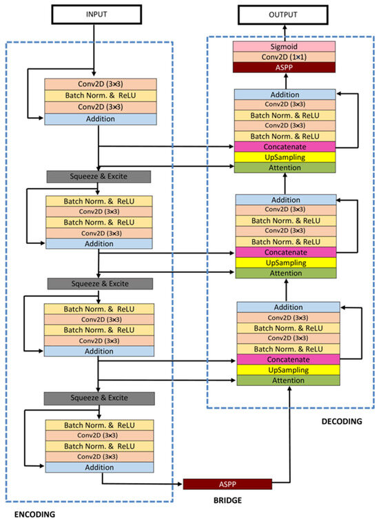
Figure 10. Schematic representation of the Attention ResU-Net ++ [88].
4.7. R2U-Net
The R2U-Net [89] model incorporates the strengths of deep residual models, Recurrent Convolutional Neural Networks (RCNN), and U-Net to deliver superior performance in segmentation tasks. The architecture of R2U-Net consists of convolutional encoding and decoding units, similar to U-Net. In the R2U-Net architecture, instead of typical forward convolutional layers, Recurrent Convolutional Layers (RCLs) and RCLs integrated with residual units are utilized within both the encoding and decoding units. The incorporation of residual units with RCLs aids in creating a more effective, deeper model. Additionally, this model features an efficient feature accumulation mechanism within the RCL units, ensuring enhanced and more robust feature representation. This is particularly beneficial for extracting very low-level features crucial for segmentation tasks. The R2U-Net distinguishes itself in three key ways: Firstly, it uses RCLs and RCLs with residual units rather than standard forward convolutional layers in both its encoding and decoding stages. Secondly, it incorporates an effective feature accumulation technique within the RCL units, enhancing feature representation. Lastly, it omits the cropping and copying unit found in the basic U-Net model, relying solely on concatenation operations, which leads to a more advanced architecture with improved performance. It also has several advantages over the U-Net model. It is efficient in terms of the number of network parameters. Although R2U-Net maintains the same quantity of network parameters as U-Net and ResU-Net, it demonstrates superior performance in segmentation tasks. The inclusion of recurrent and residual operations in R2U-Net does not augment the total number of network parameters, yet it markedly enhances both training and testing performance. The R2U-Net model’s architecture is visually represented in Figure 11.
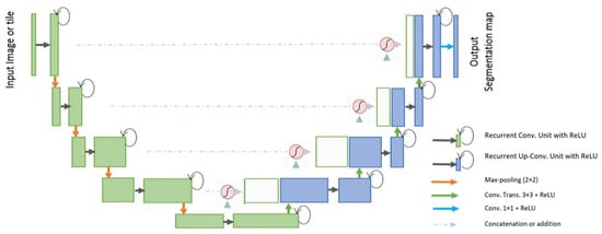
Figure 11. Schematic representation of the Attention R2U-Net [89].
4.8. nnU-Net
nnU-Net [90] is a robust tool for semantic segmentation that utilizes deep learning to automatically adapt to a given dataset. It simplifies the user experience by analyzing training cases and configuring a corresponding U-Net-based segmentation pipeline, eliminating the need for user expertise in the underlying technology.
The nnU-Net framework encompasses the entire deep learning project pipeline, from preprocessing to model configuration, training, postprocessing, and ensembling. This broad scope makes it a versatile tool for various applications. Its automatic configuration feature addresses critical components like preprocessing and network architecture.
As an open-source tool, nnU-Net delivers state-of-the-art segmentation results right out of the box. Its robustness and self-adapting framework have earned it recognition in the field of medical image segmentation and beyond. Its auto-configuration ability makes it a user-friendly solution for a wide range of segmentation tasks.
This entry is adapted from the peer-reviewed paper 10.3390/bioengineering10121349
This entry is offline, you can click here to edit this entry!